4.5. Using the ws3 optimization modelling function (advanced)

The ws3.forest.ForestMdoel class includes a number of methods to automate formulation and solution of optimization problems. In this notebook, we will demonstrate how to use these methods to formulate various common forms of objective functions and constraints, how to combine these in various ways, and how to solve these problems using the built-in solvers.

4.5.1. Set up environment

Below we (optionally) install the ws3 package from the local source code in this repository using the -e flag to ensure that the package is installed in editable mode (i.e., any changes you make to the source code immediately affect ws3 behaviour the next time you run the notebook). This is is not necessary if you have installed ws3 using pip or another method.

Note that the code in this notebook has been tested with the version of the ws3 package that is included in this repository.

Set auto-reload to reload modules when they are changed.

%load_ext autoreload
%autoreload 2

clobber_ws3 = True
if clobber_ws3:
    %pip uninstall -y ws3
    %pip install -e ..

Found existing installation: ws3 1.1.0.dev0
Uninstalling ws3-1.1.0.dev0:
  Successfully uninstalled ws3-1.1.0.dev0
Note: you may need to restart the kernel to use updated packages.
Obtaining file:///home/gep/tmp/ws3
  Installing build dependencies ... done
  Checking if build backend supports build_editable ... done
  Getting requirements to build editable ... done
  Installing backend dependencies ... done
  Preparing editable metadata (pyproject.toml) ... done
Requirement already satisfied: dill in /home/gep/tmp/ws3/.venv/lib/python3.12/site-packages (from ws3==1.1.0.dev0) (0.4.0)
Requirement already satisfied: fiona in /home/gep/tmp/ws3/.venv/lib/python3.12/site-packages (from ws3==1.1.0.dev0) (1.10.1)
Requirement already satisfied: gurobipy in /home/gep/tmp/ws3/.venv/lib/python3.12/site-packages (from ws3==1.1.0.dev0) (12.0.3)
Requirement already satisfied: highspy in /home/gep/tmp/ws3/.venv/lib/python3.12/site-packages (from ws3==1.1.0.dev0) (1.11.0)
Requirement already satisfied: libcbm in /home/gep/tmp/ws3/.venv/lib/python3.12/site-packages (from ws3==1.1.0.dev0) (2.8.1)
Requirement already satisfied: matplotlib in /home/gep/tmp/ws3/.venv/lib/python3.12/site-packages (from ws3==1.1.0.dev0) (3.10.5)
Requirement already satisfied: numpy>=1.21 in /home/gep/tmp/ws3/.venv/lib/python3.12/site-packages (from ws3==1.1.0.dev0) (2.2.6)
Requirement already satisfied: pandas>=1.3 in /home/gep/tmp/ws3/.venv/lib/python3.12/site-packages (from ws3==1.1.0.dev0) (2.3.1)
Requirement already satisfied: profilehooks in /home/gep/tmp/ws3/.venv/lib/python3.12/site-packages (from ws3==1.1.0.dev0) (1.13.0)
Requirement already satisfied: pulp in /home/gep/tmp/ws3/.venv/lib/python3.12/site-packages (from ws3==1.1.0.dev0) (3.2.2)
Requirement already satisfied: rasterio in /home/gep/tmp/ws3/.venv/lib/python3.12/site-packages (from ws3==1.1.0.dev0) (1.4.3)
Requirement already satisfied: scipy>=1.7 in /home/gep/tmp/ws3/.venv/lib/python3.12/site-packages (from ws3==1.1.0.dev0) (1.16.1)
Requirement already satisfied: python-dateutil>=2.8.2 in /home/gep/tmp/ws3/.venv/lib/python3.12/site-packages (from pandas>=1.3->ws3==1.1.0.dev0) (2.9.0.post0)
Requirement already satisfied: pytz>=2020.1 in /home/gep/tmp/ws3/.venv/lib/python3.12/site-packages (from pandas>=1.3->ws3==1.1.0.dev0) (2025.2)
Requirement already satisfied: tzdata>=2022.7 in /home/gep/tmp/ws3/.venv/lib/python3.12/site-packages (from pandas>=1.3->ws3==1.1.0.dev0) (2025.2)
Requirement already satisfied: six>=1.5 in /home/gep/tmp/ws3/.venv/lib/python3.12/site-packages (from python-dateutil>=2.8.2->pandas>=1.3->ws3==1.1.0.dev0) (1.17.0)
Requirement already satisfied: attrs>=19.2.0 in /home/gep/tmp/ws3/.venv/lib/python3.12/site-packages (from fiona->ws3==1.1.0.dev0) (25.3.0)
Requirement already satisfied: certifi in /home/gep/tmp/ws3/.venv/lib/python3.12/site-packages (from fiona->ws3==1.1.0.dev0) (2025.8.3)
Requirement already satisfied: click~=8.0 in /home/gep/tmp/ws3/.venv/lib/python3.12/site-packages (from fiona->ws3==1.1.0.dev0) (8.2.1)
Requirement already satisfied: click-plugins>=1.0 in /home/gep/tmp/ws3/.venv/lib/python3.12/site-packages (from fiona->ws3==1.1.0.dev0) (1.1.1.2)
Requirement already satisfied: cligj>=0.5 in /home/gep/tmp/ws3/.venv/lib/python3.12/site-packages (from fiona->ws3==1.1.0.dev0) (0.7.2)
Requirement already satisfied: numexpr>=2.8.7 in /home/gep/tmp/ws3/.venv/lib/python3.12/site-packages (from libcbm->ws3==1.1.0.dev0) (2.11.0)
Requirement already satisfied: numba in /home/gep/tmp/ws3/.venv/lib/python3.12/site-packages (from libcbm->ws3==1.1.0.dev0) (0.61.2)
Requirement already satisfied: pyyaml in /home/gep/tmp/ws3/.venv/lib/python3.12/site-packages (from libcbm->ws3==1.1.0.dev0) (6.0.2)
Requirement already satisfied: mock in /home/gep/tmp/ws3/.venv/lib/python3.12/site-packages (from libcbm->ws3==1.1.0.dev0) (5.2.0)
Requirement already satisfied: openpyxl in /home/gep/tmp/ws3/.venv/lib/python3.12/site-packages (from libcbm->ws3==1.1.0.dev0) (3.1.5)
Requirement already satisfied: contourpy>=1.0.1 in /home/gep/tmp/ws3/.venv/lib/python3.12/site-packages (from matplotlib->ws3==1.1.0.dev0) (1.3.3)
Requirement already satisfied: cycler>=0.10 in /home/gep/tmp/ws3/.venv/lib/python3.12/site-packages (from matplotlib->ws3==1.1.0.dev0) (0.12.1)
Requirement already satisfied: fonttools>=4.22.0 in /home/gep/tmp/ws3/.venv/lib/python3.12/site-packages (from matplotlib->ws3==1.1.0.dev0) (4.59.0)
Requirement already satisfied: kiwisolver>=1.3.1 in /home/gep/tmp/ws3/.venv/lib/python3.12/site-packages (from matplotlib->ws3==1.1.0.dev0) (1.4.8)
Requirement already satisfied: packaging>=20.0 in /home/gep/tmp/ws3/.venv/lib/python3.12/site-packages (from matplotlib->ws3==1.1.0.dev0) (25.0)
Requirement already satisfied: pillow>=8 in /home/gep/tmp/ws3/.venv/lib/python3.12/site-packages (from matplotlib->ws3==1.1.0.dev0) (11.3.0)
Requirement already satisfied: pyparsing>=2.3.1 in /home/gep/tmp/ws3/.venv/lib/python3.12/site-packages (from matplotlib->ws3==1.1.0.dev0) (3.2.3)
Requirement already satisfied: llvmlite<0.45,>=0.44.0dev0 in /home/gep/tmp/ws3/.venv/lib/python3.12/site-packages (from numba->libcbm->ws3==1.1.0.dev0) (0.44.0)
Requirement already satisfied: et-xmlfile in /home/gep/tmp/ws3/.venv/lib/python3.12/site-packages (from openpyxl->libcbm->ws3==1.1.0.dev0) (2.0.0)
Requirement already satisfied: affine in /home/gep/tmp/ws3/.venv/lib/python3.12/site-packages (from rasterio->ws3==1.1.0.dev0) (2.4.0)
Building wheels for collected packages: ws3
  Building editable for ws3 (pyproject.toml) ... done
  Created wheel for ws3: filename=ws3-1.1.0.dev0-py3-none-any.whl size=4136 sha256=5df49d1809d2f15004f3046010971c142390fb47fb3bfa7620b09e11903424a7
  Stored in directory: /tmp/pip-ephem-wheel-cache-fjqbp0j3/wheels/fa/4b/10/3fe4b92a02fb87987a6fe53a10fad0a22a781bf98cd7b63f17
Successfully built ws3
Installing collected packages: ws3
Successfully installed ws3-1.1.0.dev0
Note: you may need to restart the kernel to use updated packages.

Use pip to install Python packages listed in requirements.txt (some extra packages needed for example notebooks to run correctly).

%pip install -r requirements.txt

Requirement already satisfied: seaborn in /home/gep/tmp/ws3/.venv/lib/python3.12/site-packages (from -r requirements.txt (line 1)) (0.13.2)
Requirement already satisfied: geopandas in /home/gep/tmp/ws3/.venv/lib/python3.12/site-packages (from -r requirements.txt (line 2)) (1.1.1)
Requirement already satisfied: ipywidgets in /home/gep/tmp/ws3/.venv/lib/python3.12/site-packages (from -r requirements.txt (line 3)) (8.1.7)
Requirement already satisfied: numpy!=1.24.0,>=1.20 in /home/gep/tmp/ws3/.venv/lib/python3.12/site-packages (from seaborn->-r requirements.txt (line 1)) (2.2.6)
Requirement already satisfied: pandas>=1.2 in /home/gep/tmp/ws3/.venv/lib/python3.12/site-packages (from seaborn->-r requirements.txt (line 1)) (2.3.1)
Requirement already satisfied: matplotlib!=3.6.1,>=3.4 in /home/gep/tmp/ws3/.venv/lib/python3.12/site-packages (from seaborn->-r requirements.txt (line 1)) (3.10.5)
Requirement already satisfied: pyogrio>=0.7.2 in /home/gep/tmp/ws3/.venv/lib/python3.12/site-packages (from geopandas->-r requirements.txt (line 2)) (0.11.1)
Requirement already satisfied: packaging in /home/gep/tmp/ws3/.venv/lib/python3.12/site-packages (from geopandas->-r requirements.txt (line 2)) (25.0)
Requirement already satisfied: pyproj>=3.5.0 in /home/gep/tmp/ws3/.venv/lib/python3.12/site-packages (from geopandas->-r requirements.txt (line 2)) (3.7.1)
Requirement already satisfied: shapely>=2.0.0 in /home/gep/tmp/ws3/.venv/lib/python3.12/site-packages (from geopandas->-r requirements.txt (line 2)) (2.1.1)
Requirement already satisfied: comm>=0.1.3 in /home/gep/tmp/ws3/.venv/lib/python3.12/site-packages (from ipywidgets->-r requirements.txt (line 3)) (0.2.3)
Requirement already satisfied: ipython>=6.1.0 in /home/gep/tmp/ws3/.venv/lib/python3.12/site-packages (from ipywidgets->-r requirements.txt (line 3)) (9.4.0)
Requirement already satisfied: traitlets>=4.3.1 in /home/gep/tmp/ws3/.venv/lib/python3.12/site-packages (from ipywidgets->-r requirements.txt (line 3)) (5.14.3)
Requirement already satisfied: widgetsnbextension~=4.0.14 in /home/gep/tmp/ws3/.venv/lib/python3.12/site-packages (from ipywidgets->-r requirements.txt (line 3)) (4.0.14)
Requirement already satisfied: jupyterlab_widgets~=3.0.15 in /home/gep/tmp/ws3/.venv/lib/python3.12/site-packages (from ipywidgets->-r requirements.txt (line 3)) (3.0.15)
Requirement already satisfied: decorator in /home/gep/tmp/ws3/.venv/lib/python3.12/site-packages (from ipython>=6.1.0->ipywidgets->-r requirements.txt (line 3)) (5.2.1)
Requirement already satisfied: ipython-pygments-lexers in /home/gep/tmp/ws3/.venv/lib/python3.12/site-packages (from ipython>=6.1.0->ipywidgets->-r requirements.txt (line 3)) (1.1.1)
Requirement already satisfied: jedi>=0.16 in /home/gep/tmp/ws3/.venv/lib/python3.12/site-packages (from ipython>=6.1.0->ipywidgets->-r requirements.txt (line 3)) (0.19.2)
Requirement already satisfied: matplotlib-inline in /home/gep/tmp/ws3/.venv/lib/python3.12/site-packages (from ipython>=6.1.0->ipywidgets->-r requirements.txt (line 3)) (0.1.7)
Requirement already satisfied: pexpect>4.3 in /home/gep/tmp/ws3/.venv/lib/python3.12/site-packages (from ipython>=6.1.0->ipywidgets->-r requirements.txt (line 3)) (4.9.0)
Requirement already satisfied: prompt_toolkit<3.1.0,>=3.0.41 in /home/gep/tmp/ws3/.venv/lib/python3.12/site-packages (from ipython>=6.1.0->ipywidgets->-r requirements.txt (line 3)) (3.0.51)
Requirement already satisfied: pygments>=2.4.0 in /home/gep/tmp/ws3/.venv/lib/python3.12/site-packages (from ipython>=6.1.0->ipywidgets->-r requirements.txt (line 3)) (2.19.2)
Requirement already satisfied: stack_data in /home/gep/tmp/ws3/.venv/lib/python3.12/site-packages (from ipython>=6.1.0->ipywidgets->-r requirements.txt (line 3)) (0.6.3)
Requirement already satisfied: wcwidth in /home/gep/tmp/ws3/.venv/lib/python3.12/site-packages (from prompt_toolkit<3.1.0,>=3.0.41->ipython>=6.1.0->ipywidgets->-r requirements.txt (line 3)) (0.2.13)
Requirement already satisfied: parso<0.9.0,>=0.8.4 in /home/gep/tmp/ws3/.venv/lib/python3.12/site-packages (from jedi>=0.16->ipython>=6.1.0->ipywidgets->-r requirements.txt (line 3)) (0.8.4)
Requirement already satisfied: contourpy>=1.0.1 in /home/gep/tmp/ws3/.venv/lib/python3.12/site-packages (from matplotlib!=3.6.1,>=3.4->seaborn->-r requirements.txt (line 1)) (1.3.3)
Requirement already satisfied: cycler>=0.10 in /home/gep/tmp/ws3/.venv/lib/python3.12/site-packages (from matplotlib!=3.6.1,>=3.4->seaborn->-r requirements.txt (line 1)) (0.12.1)
Requirement already satisfied: fonttools>=4.22.0 in /home/gep/tmp/ws3/.venv/lib/python3.12/site-packages (from matplotlib!=3.6.1,>=3.4->seaborn->-r requirements.txt (line 1)) (4.59.0)
Requirement already satisfied: kiwisolver>=1.3.1 in /home/gep/tmp/ws3/.venv/lib/python3.12/site-packages (from matplotlib!=3.6.1,>=3.4->seaborn->-r requirements.txt (line 1)) (1.4.8)
Requirement already satisfied: pillow>=8 in /home/gep/tmp/ws3/.venv/lib/python3.12/site-packages (from matplotlib!=3.6.1,>=3.4->seaborn->-r requirements.txt (line 1)) (11.3.0)
Requirement already satisfied: pyparsing>=2.3.1 in /home/gep/tmp/ws3/.venv/lib/python3.12/site-packages (from matplotlib!=3.6.1,>=3.4->seaborn->-r requirements.txt (line 1)) (3.2.3)
Requirement already satisfied: python-dateutil>=2.7 in /home/gep/tmp/ws3/.venv/lib/python3.12/site-packages (from matplotlib!=3.6.1,>=3.4->seaborn->-r requirements.txt (line 1)) (2.9.0.post0)
Requirement already satisfied: pytz>=2020.1 in /home/gep/tmp/ws3/.venv/lib/python3.12/site-packages (from pandas>=1.2->seaborn->-r requirements.txt (line 1)) (2025.2)
Requirement already satisfied: tzdata>=2022.7 in /home/gep/tmp/ws3/.venv/lib/python3.12/site-packages (from pandas>=1.2->seaborn->-r requirements.txt (line 1)) (2025.2)
Requirement already satisfied: ptyprocess>=0.5 in /home/gep/tmp/ws3/.venv/lib/python3.12/site-packages (from pexpect>4.3->ipython>=6.1.0->ipywidgets->-r requirements.txt (line 3)) (0.7.0)
Requirement already satisfied: certifi in /home/gep/tmp/ws3/.venv/lib/python3.12/site-packages (from pyogrio>=0.7.2->geopandas->-r requirements.txt (line 2)) (2025.8.3)
Requirement already satisfied: six>=1.5 in /home/gep/tmp/ws3/.venv/lib/python3.12/site-packages (from python-dateutil>=2.7->matplotlib!=3.6.1,>=3.4->seaborn->-r requirements.txt (line 1)) (1.17.0)
Requirement already satisfied: executing>=1.2.0 in /home/gep/tmp/ws3/.venv/lib/python3.12/site-packages (from stack_data->ipython>=6.1.0->ipywidgets->-r requirements.txt (line 3)) (2.2.0)
Requirement already satisfied: asttokens>=2.1.0 in /home/gep/tmp/ws3/.venv/lib/python3.12/site-packages (from stack_data->ipython>=6.1.0->ipywidgets->-r requirements.txt (line 3)) (3.0.0)
Requirement already satisfied: pure-eval in /home/gep/tmp/ws3/.venv/lib/python3.12/site-packages (from stack_data->ipython>=6.1.0->ipywidgets->-r requirements.txt (line 3)) (0.2.3)
Note: you may need to restart the kernel to use updated packages.

Import required packages.

import matplotlib.pyplot as plt
import ws3
import ws3.forest
import functools
import pandas as pd

4.5.2. Set up ForestModel instance

Set some reasonable model parameters.

base_year = 2020    # base year for the problem
horizon = 10        # number of periods in the simulation horizon
period_length = 10  # period length (in years)
max_age = 1000      # maximum age of a stand (in years)
tvy_name = "totvol" # name for total volume yield component

Create a new ForestModel object and import a model dataset from the data directory.

fm = ws3.forest.ForestModel(model_name="tsa24_clipped",
                            model_path="data/woodstock_model_files_tsa24_clipped",
                            base_year=base_year,
                            horizon=horizon,
                            period_length=period_length,
                            max_age=max_age)
fm.import_landscape_section()
fm.import_areas_section(convert_periods_to_years=period_length)
fm.import_yields_section(convert_periods_to_years=period_length)
fm.import_actions_section(convert_periods_to_years=period_length)
fm.import_transitions_section(convert_periods_to_years=period_length)
fm.initialize_areas()
fm.add_null_action()
fm.reset_actions()

fm.actions["harvest"].is_harvest = True # set harvest action to be a harvest action (needed for `cmp_c_z` to work correctly)

4.5.3. Explore optimization modelling functions

4.5.3.1. Define a base scenario (maximizing harvest volume)

We will start by defining a basic optimization problem, where we simply maximize the sum of harvest volume across all time periods.

The optimization functions in ws3 are very flexible, but this flexibility comes at a cost: the user has to define various functions that generate the linear programming (LP) optimization problem matrix coefficients.

We will start by defining a function cmp_c_z (you can use any name you want for coefficient functions) that returns the objective function coefficient for a single column in the matrix. Note that ws3 is using a Model I formulation of the LP problem, where each column of the matrix represents a unique feasible combination of actions across all time periods (for a given combination of development type and initial age class). Internally ws3 handles iterating through each development type/age class combination, and generating dynamic programming state trees, where each unique path from the root node of a tree through to a leaf node is represented by a unique column in the matrix. Each path has one node per time period in the simulation horizon.

The cmp_c_z function will be used by ws3 to generate the coefficients for each column in the matrix. The cmp_c_z function takes three arguments: the first argument is a ForestModel instance, the second argument is a path (a list of node objects), and the third argument is an expr (a string expression that evaluates to a number, which we pass to the ForestModel.compile_product method).

See the ws3 documentation for more information about what types of expressions ws3 can resolve in this context. For our example we will use a simple expression that multiplies total merchantable volume in the totvol yield component by 0.85 to simulate an 85% fibre utilization rate (i.e., 15% of total merchnantable volume is left behind as harvest residues in slash piles or spread across cut blocks).

The Model I LP optimization problem can be formulated as follows:

\[\begin{split}\begin{align} \text{max} \quad & \sum_{i\in I}\sum_{j \in J_{i}}c_{ij}x_{ij} & \\ \text{s.t.} \quad & \nonumber \\ &(1-\varepsilon_{p})y_p \leq \sum_{i\in I}\sum_{j\in J_{i}}\mu_{ijpt}x_{ij} \leq (1+\varepsilon_{p})y_p, & \forall p\in O', t\in T'_p \\ &v^{-}_{ot}\leq\sum_{i\in Z}\sum_{j\in J_{i}}\mu_{ijot}x_{ij} \leq v^{+}_{ot}, & \forall o\in O, t\in T \\ &\sum_{j\in J_{i}}x_{ij} = 1, \forall i\in Z \\ &0 \leq x_{ij} \leq 1, & \forall i \in Z, j \in J_{i} \end{align}\end{split}\]

where

\[\begin{split}\begin{align*} I := & \,\, \text{set of spatial zones}\\ J_{i} := & \,\, \text{set of available prescriptions for zone $i \in I$}\\ O := & \,\, \text{set of forest outputs}\\ O' \subseteq O := & \,\, \text{set of targeted forest outputs}\\ T := & \,\, \text{set of time periods in the planning horizon}\\ T'_p \subseteq O := & \,\, \text{subset of $T$ on which even-flow constraints for output $p \in O^{\prime}$ are applied}\\ \varepsilon_{p} := & \,\, \text{admissible level of variation on yield of targeted output $p \in O^{\prime}$} \\ \mu_{ijot} := & \,\, \text{quantity of output $o \in O$ produced in period $t \in T$ by prescription $j \in J_{i}$}\\ & \,\, \text{in zone $i \in I$}\\ \mu_{ijpt} := & \,\, \text{quantity of output $p \in O'$ produced in period $t \in T$ by prescription $j \in J_{i}$}\\ & \,\, \text{in zone $i \in I$}\\ v^{-}_{ot} := & \,\, \text{lower bound on yield of output $o \in O$ in period $t \in T$} \\ v^{+}_{ot} := & \,\, \text{upper bound on yield of output $o \in O$ in period $t \in T$} \\ c_{ij} := & \,\, \text{objective function contribution of prescription $j \in J_{i}$ in zone $i \in I$} \\ x_{ij} := & \,\, \text{proportion of zone $i \in Z$ on which prescription $j \in J_{i}$ is applied} \\ y_p = & \sum_{i\in I}\sum_{j\in J_i}\mu_{ijpt^R_p}x_{ij}\text{, i.e. total yield of targeted output $p \in O'$ at reference period $t^R_p$} \end{align*}\end{split}\]

The objective function (1) maximizes the sum of \(c_{ij}x_{ij}\) products, which represent yield of a user-defined output—the output can be anything, but will typically be harvest volume or harvested area.

The variables \(x_{ij}\) are linear, with domain \(\{x_{ij} \in \mathbb{R}|0 \leq x_{ij} \leq 1\}\) specified in (5).

The set \(O^{\prime} \subseteq O\) represents targeted outputs, for which we enforce even-flow constraints. Even-flow constraints are defined in (2), and are expressed in terms of \(y_p\), which represents total yield of targeted output \(p \in O^{\prime}\) in reference period \(t^R_p\). Note that even-flow constraints are defined over time periods \(T'_p\), which is any subset of \(T\) (need not be contiguous)—\(T'_p\) can be unique for each output \(p \in O^{\prime}\).

General constraints (3) set upper and lower bounds on periodic yield of any output \(o \in O\)—we can use these constraints to set minimum or maximum periodic levels of any indicators that we can formulate from data in the model (e.g., set an upper bount on harvest volume in the first period, or set a lower bound on growing stock in the final period).

Coverage constraints (4) are accounting constraints that force prescriptions to cover the entire zone—doing nothing for the entire planning horizon is considered a prescription that could generate some outputs. This maintains the structure of the model, and these are automatically defined and set by ws3 (i.e., the user does not need to define these constraints as part of optimization model input).

def cmp_c_z(fm, path, expr):
    """
    Compile objective function coefficient (given ForestModel instance,
    root-to-leaf state tree node path, and an expression that resolves to the correct product unit).

    This function iterates over the specified node path in a state tree,
    checks if each node corresponds to a harvest operation, and adds up the compiled product values for these nodes.

    Parameters:
    fm (ForestModel): The ForestModel instance containing the necessary information.
    path (list of Node objects): A list of root-to-leaf nodes forming a path through a state tree.
    expr (str): An expression resolving to the correct product unit.

    Returns:
    float: The compiled objective function coefficient.
    """
    result = 0. # Initialize the result variable
    for t, n in enumerate(path, start=1): # Iterate over the node path with index and value
        d = n.data() # Get the data from the current node
        if fm.is_harvest(d["acode"]): # Check if the current node corresponds to a harvest operation
            result += fm.compile_product(t, expr, d["acode"], [d["dtk"]], d["age"], coeff=False) # Add up the compiled product values
    return result # Return the final compiled objective function coefficient

Note that a decision variables in the Model I problem represents a proportion of the total area in a given tree that is assigned to a given path (sequence of actions), and that the sum of all decision variables corresponding to a given tree is automatically constrained to sum to 1. As such, the objective function coefficients should represent absolute yield (e.g., \(m^3\) for harvest volume, not \(m^3 ha^{-1}\)).

Next we define the coeff_funcs dictionary, which maps matrix row names to the functions that we defined that generate the correct coefficients for each column of the matrix in that row. In this simple we only map row z names to the cmp_c_z function that we defined above. This tells the ForestModel.add_problem method to use the cmp_c_z function to compile the objective function coefficients (the objective function is named z by default in the ForestModel.add_problem method arg signature definition, so if we map a function to name z in coeff_funcs it will automatically pick that up as the objective function coefficient function).

Note that the add_problem method assumes that all coefficient functions passed to coeff_funcs will have exactly two arguments (a ForestModel instance and a Path instance). If this is not the case then you will need to define a wrapper function that rewrites the function signature (see the example below using functools.partial).

expr = "0.85 * totvol"
coeff_funcs = {"z":functools.partial(cmp_c_z, expr=expr)}

Now we are ready to call the ForestModel.add_problem method, which will build the optimization problem (including the objective function coefficients from the function we provided) and add the problem to the model under the name 'scenario-1'. The add_problem method returns an instance of the Problem class that we can use to solve the LP problem and access the optimal solution (which we will compile into a ws3 action schedule so we can simulate it out and plot results in a human-readable way).

We pass None value to the cflw_e and cgen_data arguments because there are no flow or general constraints in this problem.

We pass 'null' and 'harvest' values to the acodes argument because these are the action we want to include in the generation of the Model 1 state trees in this problem. This allows us to define complex ForestModel base models, which potentially define a wide range of actions, without being required to always include all the defined actions in all the optimization problems. It is required to define a null action in the ForestModel instance before calling the add_problem method (the ForestModel.add_null_action method makes it easy to correctly define a null action), and you must include the name of the null action in the list of action codes passed to the acodes argument of the add_problem method. Including a null action allows the optimization problem to simulate doing nothing (i.e., just letting the forest grow). If you want to include all the actions defined in the ForestModel, pass None value to the acodes argument of the add_problem method.

We pass None to the mask argument because we want to include all the development types in this problem. You can filter which developments are included in a given problem by passing a valid mask (either in tuple format or as a Woodstock-style mask string). See the ws3 documentation for more information about themes and masks (including how to define aggregate landscape codes to match multiple values within one theme in a mask).

Note also that the objective function sense gets defined at this point by passing the sense argument to the add_problem method. The sense argument can be either ws3.opt.SENSE_MINIMIZE or ws3.opt.SENSE_MAXIMIZE.

problem = fm.add_problem(name="scenario-1",
                         coeff_funcs=coeff_funcs,
                         cflw_e=None,
                         cgen_data=None,
                         acodes=("null", "harvest"),
                         sense=ws3.opt.SENSE_MAXIMIZE,
                         mask=None)

Now that we have a Problem object instance, we can call the solve method to try to solve the problem.

This will use the default bindings to the open source HiGHS solver (see the HiGHS documentation for details on HiGHS) to find a solution that maximizes the objective.

problem.solve(verbose=True)

Running HiGHS 1.11.0 (git hash: 364c83a): Copyright (c) 2025 HiGHS under MIT licence terms
LP   has 32 rows; 305 cols; 305 nonzeros
Coefficient ranges:
  Matrix [1e+00, 1e+00]
  Cost   [2e+01, 4e+04]
  Bound  [1e+00, 1e+00]
  RHS    [1e+00, 1e+00]
Presolving model
24 rows, 115 cols, 115 nonzeros  0s
0 rows, 0 cols, 0 nonzeros  0s
Presolve : Reductions: rows 0(-32); columns 0(-305); elements 0(-305) - Reduced to empty
Solving the original LP from the solution after postsolve
Using EKK primal simplex solver
  Iteration        Objective     Infeasibilities num(sum)
          0    -2.2455249290e+05 Pr: 0(0); Du: 222(1.63573e+06) 0s
         19    -2.2455284502e+05 Pr: 0(0) 0s
Required 19 simplex iterations after postsolve
Model status        : Optimal
Simplex   iterations: 19
Objective value     : -2.2455284502e+05
P-D objective error :  6.4803823015e-17
HiGHS run time      :          0.00

We can use the Problem.status method to check the status of the solution (i.e., to confirm that the problem was solved to optimality).

if (problem.status() == ws3.opt.STATUS_OPTIMAL):
    print("Hooray! We have an optimal solution!")

Hooray! We have an optimal solution!

We can use the Problem.z method to check the value of the objective function at the optimal solution.

print("The optimal value of the objective function is: {}".format(problem.z()))

The optimal value of the objective function is: 224552.84502455403

This matches the value reported by HiGHS in the solver stdout console output in a previous step.

Next, we need to extract the optimal sequence of actions from the Problem instance and compile it into a format that can be used as input to the ForestModel.apply_schedule method. We can use the ForestModel.compile_schedule method to do this. Internally this dispatches the call to private method ForestModel._cmp_sch_m1, which is aware of the Model I optimization problem structure and correctly walks through all the Node objects in all the Path objects in all the Tree objects in the Problem instance that was passed in as an argument, extracting the required data (i.e., DevelopmentType key, age, actionned area, action code, period, existing/future DevelopmentType status) from the data dictionary of each Node object and assembling this information into a correctly formatted list of tuples that can be consumed by ForestModel.apply_action.

schedule = fm.compile_schedule(problem)
schedule

[(('tsa24_clipped', '1', '2401002', '204', '2401002'),
  85,
  282.1296355046733,
  'harvest',
  1,
  '_existing'),
 (('tsa24_clipped', '1', '2401002', '204', '2401002'),
  91,
  73.1021561503533,
  'harvest',
  1,
  '_existing'),
 (('tsa24_clipped', '1', '2401002', '204', '2401002'),
  93,
  28.37956666951611,
  'harvest',
  1,
  '_existing'),
 (('tsa24_clipped', '1', '2401002', '204', '2401002'),
  95,
  94.94675966211176,
  'harvest',
  1,
  '_existing'),
 (('tsa24_clipped', '1', '2401002', '204', '2401002'),
  105,
  32.175418531537815,
  'harvest',
  1,
  '_existing'),
 (('tsa24_clipped', '1', '2401002', '204', '2401002'),
  113,
  4.184826329641321,
  'harvest',
  1,
  '_existing'),
 (('tsa24_clipped', '1', '2401002', '204', '2401002'),
  115,
  50.030816858894816,
  'harvest',
  1,
  '_existing'),
 (('tsa24_clipped', '1', '2401002', '204', '2401002'),
  125,
  78.16612132001225,
  'harvest',
  1,
  '_existing'),
 (('tsa24_clipped', '1', '2401002', '204', '2401002'),
  135,
  72.24421919373785,
  'harvest',
  1,
  '_existing'),
 (('tsa24_clipped', '1', '2401002', '204', '2401002'),
  145,
  96.38442685503642,
  'harvest',
  1,
  '_existing'),
 (('tsa24_clipped', '1', '2401002', '204', '2401002'),
  153,
  9.591469412607397,
  'harvest',
  1,
  '_existing'),
 (('tsa24_clipped', '1', '2401002', '204', '2401002'),
  155,
  34.32629241113743,
  'harvest',
  1,
  '_existing'),
 (('tsa24_clipped', '1', '2402000', '100', '2402000'),
  165,
  0.638005468748551,
  'harvest',
  1,
  '_existing'),
 (('tsa24_clipped', '1', '2402002', '204', '2402002'),
  93,
  48.21816452980633,
  'harvest',
  1,
  '_existing'),
 (('tsa24_clipped', '1', '2402002', '204', '2402002'),
  95,
  33.89498244313859,
  'harvest',
  1,
  '_existing'),
 (('tsa24_clipped', '1', '2402002', '204', '2402002'),
  115,
  3.195378954654358,
  'harvest',
  1,
  '_existing'),
 (('tsa24_clipped', '1', '2403000', '100', '2403000'),
  93,
  14.811643286926836,
  'harvest',
  1,
  '_existing'),
 (('tsa24_clipped', '1', '2402002', '204', '2402002'),
  88,
  32.64168183055375,
  'harvest',
  2,
  '_existing'),
 (('tsa24_clipped', '1', '2403002', '204', '2403002'),
  83,
  2.243990590272984,
  'harvest',
  2,
  '_existing'),
 (('tsa24_clipped', '1', '2401002', '204', '2401002'),
  168,
  103.76740323520823,
  'harvest',
  10,
  '_existing'),
 (('tsa24_clipped', '1', '2401002', '204', '2401002'),
  170,
  4.173147018452507,
  'harvest',
  10,
  '_existing'),
 (('tsa24_clipped', '1', '2401002', '204', '2421002'),
  90,
  282.1296355046733,
  'harvest',
  10,
  '_existing'),
 (('tsa24_clipped', '1', '2401002', '204', '2421002'),
  90,
  73.1021561503533,
  'harvest',
  10,
  '_existing'),
 (('tsa24_clipped', '1', '2401002', '204', '2421002'),
  90,
  28.37956666951611,
  'harvest',
  10,
  '_existing'),
 (('tsa24_clipped', '1', '2401002', '204', '2421002'),
  90,
  94.94675966211176,
  'harvest',
  10,
  '_existing'),
 (('tsa24_clipped', '1', '2401002', '204', '2421002'),
  90,
  32.175418531537815,
  'harvest',
  10,
  '_existing'),
 (('tsa24_clipped', '1', '2401002', '204', '2421002'),
  90,
  4.184826329641321,
  'harvest',
  10,
  '_existing'),
 (('tsa24_clipped', '1', '2401002', '204', '2421002'),
  90,
  50.030816858894816,
  'harvest',
  10,
  '_existing'),
 (('tsa24_clipped', '1', '2401002', '204', '2421002'),
  90,
  78.16612132001225,
  'harvest',
  10,
  '_existing'),
 (('tsa24_clipped', '1', '2401002', '204', '2421002'),
  90,
  72.24421919373785,
  'harvest',
  10,
  '_existing'),
 (('tsa24_clipped', '1', '2401002', '204', '2421002'),
  90,
  96.38442685503642,
  'harvest',
  10,
  '_existing'),
 (('tsa24_clipped', '1', '2401002', '204', '2421002'),
  90,
  9.591469412607397,
  'harvest',
  10,
  '_existing'),
 (('tsa24_clipped', '1', '2401002', '204', '2421002'),
  90,
  34.32629241113743,
  'harvest',
  10,
  '_existing'),
 (('tsa24_clipped', '1', '2401002', '204', '2421002'),
  110,
  0.422054121206099,
  'harvest',
  10,
  '_existing'),
 (('tsa24_clipped', '1', '2402000', '100', '2422000'),
  90,
  0.638005468748551,
  'harvest',
  10,
  '_existing'),
 (('tsa24_clipped', '1', '2402002', '204', '2422002'),
  80,
  32.64168183055375,
  'harvest',
  10,
  '_existing'),
 (('tsa24_clipped', '1', '2402002', '204', '2422002'),
  90,
  48.21816452980633,
  'harvest',
  10,
  '_existing'),
 (('tsa24_clipped', '1', '2402002', '204', '2422002'),
  90,
  33.89498244313859,
  'harvest',
  10,
  '_existing'),
 (('tsa24_clipped', '1', '2402002', '204', '2422002'),
  90,
  3.195378954654358,
  'harvest',
  10,
  '_existing'),
 (('tsa24_clipped', '1', '2403000', '100', '2423000'),
  90,
  14.811643286926836,
  'harvest',
  10,
  '_existing'),
 (('tsa24_clipped', '1', '2403002', '204', '2423002'),
  80,
  2.243990590272984,
  'harvest',
  10,
  '_existing'),
 (('tsa24_clipped', '1', '2403002', '204', '2423002'),
  99,
  59.81429119367274,
  'harvest',
  10,
  '_existing'),
 (('tsa24_clipped', '1', '2403002', '204', '2423002'),
  108,
  32.366198551219505,
  'harvest',
  10,
  '_existing')]

As you can see, the schedule is just a list of 6-element tuples.

The first element in each tuple is the DevelopmentType key (a tuple of landscape theme strings).

The other elements in the tuple specify the age, actionned area, action code, period, and existing/future DevelopmentType status.

Now we that we have a compiled schedule, we can use it as input for the ForestModel.apply_schedule method using the following parameters:

• force_integral_area: Set to False to avoid forcing integral area calculations

• override_operability: Set to False to avoid overriding operability calculations

• fuzzy_age: Set to False to disable fuzzy age calculations

• recourse_enabled: Set to False to disable recourse-enabled mode

• verbose: Set to False for quiet operation

• compile_c_ycomps: Set to True to enable compilation of complex yield components

See the ws3 documentation for the ForestModel.apply_schedule and ForestModel.apply_action methods for more information about these and other parameters that are available to controls exactly how actions get applied to the model. Ultimately, the apply_schedule method is a wrapper around the apply_action method. The apply_action method will handle the details of applying individual actions to the model. One of the main functions of ws3 (and any forest estate model) is to simulate forest response to sequences of actions interleaved with periods of growth. Given the core role of the apply_action method, it is not surprising that it has a large number of parameters that can be used to control exactly how actions are applied.

This effectively resets the current schedule and model state to the initial state, and runs a sequential multi-period simulation of alternating actions and periods of growth.

fm.apply_schedule(
    schedule,
    force_integral_area=False,
    override_operability=False,
    fuzzy_age=False,
    recourse_enabled=False,
    verbose=False,
    compile_c_ycomps=True
)

0.0

At this point, our ForestModel object has simulated sequential application of the optimal schedule of activities we created in a previous step.

Next, we compile some relevant performance indicators to summarize what is going in this optimal solution (i.e., periodic harvested area, periodic harvest volume, periodic growing stock).

First, we compile the harvested area and volume indicators. We use the ForestModel.ompile_product method to compile these indicators. The first argument is the period for which we want to compile a product output, while the second argument is the expression that will be resolved by ws3 to compute a yield coefficient. The compile_product method compiles the product of actionned area and whatever yield coefficient the provided expression resolves to (expressed in units of output product per unit of area, e.g., \(m^3/ha\) for harvested volume or \(ha/ha\) for harvested area). So, when we use an expression value of 1. for the second argument of the compile_product method, we are telling ws3 that we want to pass through the actionned area indicator that it is calculating internally. We use the acode argument to specify which action code to use (i.e., harvest to compile harvested area and harvested volume indicators).

We use the ForestModel.inventory method to compile the growing stock indicator. The first argument is the period for which we want to compile an inventory output, while the second argument is the expression that will be resolved by ws3 to compute a yield coefficient (in this case we use the total volume of trees multiplied by an assumed utilization rate of 85%).

See the ws3 documentation for more information on expression evaluation, and what types of expressions are supported by ws3 that can be provided as input to compile_product and inventory method calls.

Once we have compiled our raw indictor outputs into lists (with one value period, including a data column of period index values), we stuff all of this into a dictionary and create a new pandas.DataFrame to hold our compiled data.

oha = [fm.compile_product(period, "1.", acode="harvest") for period in fm.periods]
ohv = [fm.compile_product(period, "totvol * 0.85", acode="harvest") for period in fm.periods]
ogs = [fm.inventory(period, "totvol") for period in fm.periods]
data = {"period":fm.periods,
        "oha":oha,
        "ohv":ohv,
        "ogs": ogs}
df = pd.DataFrame(data)
df

	period	oha	ohv	ogs
0	1	956.419884	102585.020390	30405.125309
1	2	34.885672	4798.494437	28607.304394
2	3	0.000000	0.000000	32154.392350
3	4	0.000000	0.000000	38166.885368
4	5	0.000000	0.000000	47379.394949
5	6	0.000000	0.000000	59578.656570
6	7	0.000000	0.000000	77531.535059
7	8	0.000000	0.000000	103522.146540
8	9	0.000000	0.000000	134548.020901
9	10	1191.848650	117169.330197	25643.073440

Plot this data as bar charts using matplotlib.

fig, ax = plt.subplots(1, 3, figsize=(12, 4))
ax[0].bar(df.period, df.oha)
ax[0].set_ylim(0, None)
ax[0].set_title("Harvested area (ha)")
ax[1].bar(df.period, df.ohv)
ax[1].set_ylim(0, None)
ax[1].set_title("Harvested volume (m3)")
ax[2].bar(df.period, df.ogs)
ax[2].set_ylim(0, None)
ax[2].set_title("Growing Stock (m3)")
fig, ax

(<Figure size 1200x400 with 3 Axes>,
 array([<Axes: title={'center': 'Harvested area (ha)'}>,
        <Axes: title={'center': 'Harvested volume (m3)'}>,
        <Axes: title={'center': 'Growing Stock (m3)'}>], dtype=object))

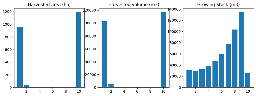
So, the optimal solution seems to be to harvest a lot of volume in the first period, then just let the forest grow for 90 years, then liquidate all operable growing stock in the final period.

This is typical behaviour for a forest estate model when there are no even flow or growing stock constraints defined. This is a good example of why it is essential for the forest analyst formulating and solving LP optimization problems in a forest estate modelling environment to understand the four inherent assumptions of linear programming (i.e., proportionality, additivity, divisibility, and certainty). In this case, the certainty assumption is relevant to understanding the behaviour of the model. The model is certain that time ends after perido 10, and is therefore certain that there is no reason to maintain any growing stock (hence the determination that the optimal policy is to liquidate all remaining operable growing stock before time ends).

The analyst needs to understand the effect of these assumptions on model output, and to detect when externalities need to be dealt with to mitigate any perverse effects of model structure and formulation. This is why experienced analysts might set a lower bound constraint on final-period growing stock, as a proxy for future time steps (beyond the final period in the model) that that model does not (cannot because of the certainty assumption) see. This is a common practice in forest estate modelling, so we will go ahead and model this in the next step.

4.5.3.2. Adding a Lower Bound Constraint on Final Period Growing Stock

Next we will set such a lower bound constraint on final period growing stock, and re-run the model.

Before settting this new constraint, we need to define new function that correctly calculates the optimization problem matrix coefficients for the new constraint rows.

def cmp_c_ci(fm, path, yname, mask=None): # product, named actions
    """
    Compile constraint coefficient for inventory indicator.

    This function takes a ForestModel instance and other parameters to evaluate
    an expression along a specified leaf-to-root-node path. It returns a dictionary
    where keys are timestamps (t) and values are the results of evaluating the given
    expression at each timestamp, with optional filtering based on the provided mask.

    Parameters:
        fm (ForestModel): The ForestModel instance to use for evaluation.
        path: A list of nodes representing one path in one tree in the optimization problem.
        yname (str): The name of the yield component used for output coefficient lookup.
        mask (tuple or string, optional): An optional dictionary that specifies which data types
            should be used for filtering.

    Returns:
        dict: A dictionary where keys are timestamps and values are the constraint coefficients for the matrix.
    """
    result = {}
    # Iterate over each node in the specified path
    for t, n in enumerate(path, start=1):
        d = n.data()
        if mask and not fm.match_mask(mask, d["_dtk"]): continue # filter by mask
        result[t] = fm.inventory(t, yname=yname, age=d["_age"], dtype_keys=[d["_dtk"]])
    return result

Now we can use the functools.partial function to create a new version of the cmp_c_i function that takes two arguments (i.e., a ForestModel instance and a tuple of Node objects), and map this to constraint name cgen_gs in the coeff_funcs dictionary (which already contains a mapping to the objective function coefficient function, from a previous step).

coeff_funcs['cgen_gs'] = functools.partial(cmp_c_ci, yname=tvy_name, mask=None)

Next we need to create the cgen_data argument for the ForestModel.add_problem method, which is a data structure that contains periodic lower-bound and upper-bound right-hand-side (RHS) values that we will be used to define the new end-of-horizon minimum growing stock constraint.

We can use the ForestModel.inventory method to query the model for initial growing stock level, so we can set the ending inventory constraint to 90% of this initial value.

gs_lb_rhs = fm.inventory(0, "totvol") * 0.90 # 90% of initial growing stock level
cgen_data = {"cgen_gs":{"lb":{10:gs_lb_rhs}, "ub":{10:999999999.}}}
cgen_data

{'cgen_gs': {'lb': {10: 135984.04613242325}, 'ub': {10: 999999999.0}}}

The cgen_data argument to ForestestModel.add_problem is a dictionary that contains constraint names as keys and dictionaries with keys lb (lower bound RHS values) and ub (upper bound RHS values) as values. The RHS values are also dictionaries, where each key is a period and value is the RHS value for that age. In this case we will only define RHS values for period 10. We set the he lower bound RHS value for period 10 as 90% of initial growing stock level and the upper bound RHS value for period 10 as 999999999 (an arbitrary large number, as we want the upper bound to be a non-binding constraint). We will use these values to define the new end-of-horizon minimum growing stock.

We can now add the new constraint using the add_problem method. The call to add_problem is almost identical to that of add_problem for the first scenario. The only difference is that we pass the new cgen_data object(containing lower-bound and upper-bound constraint RHS values) instead of passing None and that the coeff_funcs dictionary now also includes a key-value pair for the new coefficient function we defined to track periodic growing stock inventory.

problem = fm.add_problem(name="scenario-2",
                         coeff_funcs=coeff_funcs,
                         cflw_e=None,
                         cgen_data=cgen_data, # this was set to None in the previous scenario
                         acodes=("null", "harvest"),
                         sense=ws3.opt.SENSE_MAXIMIZE,
                         mask=None)

Now we can solve our upgraded problem, compile and simulate the optimal solution, and display results. Note that we need to call ForestModel.reset() before applying the new action schedule (other wise ws3 will just attempt to apply the actions on top of previously applied actions, which will simulate the wrong scenario and give you incorrect results).

problem.solve()
sch = fm.compile_schedule(problem)
fm.reset()
fm.apply_schedule(
    sch,
    force_integral_area=False,
    override_operability=False,
    fuzzy_age=False,
    recourse_enabled=False,
    verbose=False,
    compile_c_ycomps=True
)
oha = [fm.compile_product(period, "1.", acode="harvest") for period in fm.periods]
ohv = [fm.compile_product(period, "totvol * 0.85", acode="harvest") for period in fm.periods]
ogs = [fm.inventory(period, "totvol") for period in fm.periods]
data = {
    "period":fm.periods,
    "oha":oha,
    "ohv":ohv,
    "ogs":ogs
}
df = pd.DataFrame(data)
fig, ax = plt.subplots(1, 3, figsize=(12, 4))
ax[0].bar(df.period, df.oha)
ax[0].set_ylim(0, None)
ax[0].set_title("Harvested area (ha)")
ax[1].bar(df.period, df.ohv)
ax[1].set_ylim(0, None)
ax[1].set_title("Harvested volume (m3)")
ax[2].bar(df.period, df.ogs)
ax[2].set_ylim(0, None)
ax[2].set_title("Growing Stock (m3)")
fig, ax

(<Figure size 1200x400 with 3 Axes>,
 array([<Axes: title={'center': 'Harvested area (ha)'}>,
        <Axes: title={'center': 'Harvested volume (m3)'}>,
        <Axes: title={'center': 'Growing Stock (m3)'}>], dtype=object))

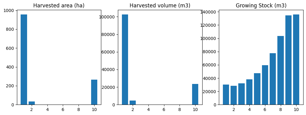
That is a bit better. At least we are not liquidating our growing stock at the ned of the simulation horizon anymore. It would be nice to reduce variation in the periodic harvest volume, however. We achieve this by adding an even flow constraint to the model.

In the next section, We are going extend and resolve our model a few more times after this, but first we can define a new run_scenario function that will take care of this and avoid having this notebook fill up with mostly cut-and-paste repeated blocks of code. The function includes cleaned up code blocks that replicate all the things we manually implemented in previous steps, but all linked together.

Note how we defined two Python closures inside run_scenario (compile_scenario and plot_scenario) to handle compiling and plotting solutions. Before moving on to adding even flow constraints to our model, we will test out our new run_scenario function and explore how its arguments affect how the model is built and what data is output to the console.

def run_scenario(forest_model, scenario_name, sense, acodes, coeff_funcs, cflw_e, cgen_data,
                 solver=ws3.opt.SOLVER_HIGHS, verbose=False, workers=1):
    """
    Runs a forest management scenario using the provided forest model.

    Parameters:
        forest_model (object): The forest model to use for this scenario.
        scenario_name (str): A name for this scenario.
        sense (str): The optimization sense for this scenario ("minimize" or "maximize").
        coeff_funcs (list of functions): Functions that define the coefficients for this scenario.
        cflw_e (float): The cost of flow-out for this scenario.
        cgen_data (dict): Data for generation in this scenario.
        acodes (list of str): Codes for acres to include in this scenario.
        solver (str, optional): The solver to use for this scenario. Defaults to ws3.opt.SOLVER_PULP.

    Returns:
        fig: A matplotlib figure with plots of harvested area, volume, and growing stock.
        df: A pandas DataFrame containing the compiled scenario data.
        problem: The optimization problem object used in this scenario.
    """

    # Helper function to compile scenario data
    def compile_scenario(fm):
        """
        Compiles scenario data for a given forest model.

        Parameters:
            fm (object): The forest model to use for compilation.

        Returns:
            df: A pandas DataFrame containing the compiled scenario data.
        """
        # Compile product harvest area and volume for each period in the forest model
        oha = [fm.compile_product(period, "1.", acode="harvest") for period in fm.periods]
        ohv = [fm.compile_product(period, "totvol * 0.85", acode="harvest") for period in fm.periods]

        # Get the growing stock inventory for each period in the forest model
        ogs = [fm.inventory(period, "totvol") for period in fm.periods]

        # Create a dictionary to hold the compiled data and convert it to a DataFrame
        data = {"period": fm.periods,
                "oha": oha,
                "ohv": ohv,
                "ogs": ogs}
        df = pd.DataFrame(data)

        return df

    # Helper function to plot scenario data
    def plot_scenario(df):
        """
        Plots the harvested area, volume, and growing stock for a given scenario.

        Parameters:
            df (pandas DataFrame): The compiled scenario data to plot.
        """
        fig, ax = plt.subplots(1, 3, figsize=(12, 4))

        # Plot harvested area
        ax[0].bar(df.period, df.oha)
        ax[0].set_ylim(0, None)
        ax[0].set_title("Harvested Area (ha)")

        # Plot harvested volume
        ax[1].bar(df.period, df.ohv)
        ax[1].set_ylim(0, None)
        ax[1].set_title("Harvested Volume (m3)")

        # Plot growing stock
        ax[2].bar(df.period, df.ogs)
        ax[2].set_ylim(0, None)
        ax[2].set_title("Growing Stock (m3)")

        return fig, ax

    # Create the optimization problem for this scenario
    problem = forest_model.add_problem(name=scenario_name,
                                       coeff_funcs=coeff_funcs,
                                       cflw_e=cflw_e,
                                       cgen_data=cgen_data,
                                       acodes=acodes,
                                       sense=sense,
                                       mask=None,
                                       verbose=verbose,
                                       workers=workers)

    # Set the solver and solve the optimization problem
    problem.solver(solver)
    forest_model.reset()
    problem.solve(verbose=verbose)

    if problem.status() != ws3.opt.STATUS_OPTIMAL:
        print("Model not optimal.")
        df = None
        fig = None
    else:
        # Compile schedule from optimization problem
        schedule = forest_model.compile_schedule(problem)

        # Apply compiled schedule to the forest model
        forest_model.apply_schedule(schedule,
                                    force_integral_area=False,
                                    override_operability=False,
                                    fuzzy_age=False,
                                    recourse_enabled=False,
                                    verbose=False,
                                    compile_c_ycomps=True)

        # Re-compile scenario data with new schedule applied
        df = compile_scenario(forest_model)

        # Plot the compiled scenario data
        fig, ax = plot_scenario(df)
    return fig, df, problem

Now we can easily formulate and solve an optimization problem, compile an action schedule from the optimal solution and simulate it in ws3, and plot results.

acodes = ["null", "harvest"]
run_scenario(fm, "scenario-2", ws3.opt.SENSE_MAXIMIZE, acodes, coeff_funcs, None, cgen_data)

(<Figure size 1200x400 with 3 Axes>,
    period         oha            ohv            ogs
 0       1  956.419884  102585.020390   30405.125309
 1       2   34.885672    4798.494437   28607.304394
 2       3    0.000000       0.000000   32154.392350
 3       4    0.000000       0.000000   38166.885368
 4       5    0.000000       0.000000   47379.394949
 5       6    0.000000       0.000000   59578.656570
 6       7    0.000000       0.000000   77531.535059
 7       8    0.000000       0.000000  103522.146540
 8       9    0.000000       0.000000  134548.020901
 9      10  266.188474   23379.503408  135984.046132,
 <ws3.opt.Problem at 0x74e8c151efc0>)

This new function will allow us to easily run several different scenarios. We can also easily add new scenarios to the model by simply changing the input parameters and observing how it affects model output and behaviour.

Note that our new run_scenario function includes a verbose arg that we can use to to print out more information as ws3 formulates and solves a new optimization problem.

acodes = ["null", "harvest"]
run_scenario(fm, "scenario-2", ws3.opt.SENSE_MAXIMIZE, acodes, coeff_funcs, None, cgen_data, verbose=True)

add_problem: build problem
generate trees using 1 workers
process trees
_bld_p_m1: build problem
_bld_p_m1: done building problem
add_problem: compile flow constraints
add_problem: compile general constraints
Running HiGHS 1.11.0 (git hash: 364c83a): Copyright (c) 2025 HiGHS under MIT licence terms
LP   has 34 rows; 305 cols; 585 nonzeros
Coefficient ranges:
  Matrix [1e+00, 5e+04]
  Cost   [2e+01, 4e+04]
  Bound  [1e+00, 1e+00]
  RHS    [1e+00, 1e+09]
Presolving model
25 rows, 218 cols, 350 nonzeros  0s
22 rows, 151 cols, 280 nonzeros  0s
Dependent equations search running on 21 equations with time limit of 1000.00s
Dependent equations search removed 0 rows and 0 nonzeros in 0.00s (limit = 1000.00s)
22 rows, 151 cols, 280 nonzeros  0s
Presolve : Reductions: rows 22(-12); columns 151(-154); elements 280(-305)
Solving the presolved LP
Using EKK parallel dual simplex solver - SIP with concurrency of 8
  Iteration        Objective     Infeasibilities num(sum)
          0     0.0000000000e+00 Ph1: 0(0) 0s
         39    -1.3076301824e+05 Pr: 0(0); Du: 0(4.26326e-13) 0s
Solving the original LP from the solution after postsolve
Model status        : Optimal
Simplex   iterations: 39
Objective value     : -1.3076301824e+05
P-D objective error :  5.5642106547e-17
HiGHS run time      :          0.00

(<Figure size 1200x400 with 3 Axes>,
    period         oha            ohv            ogs
 0       1  956.419884  102585.020390   30405.125309
 1       2   34.885672    4798.494437   28607.304394
 2       3    0.000000       0.000000   32154.392350
 3       4    0.000000       0.000000   38166.885368
 4       5    0.000000       0.000000   47379.394949
 5       6    0.000000       0.000000   59578.656570
 6       7    0.000000       0.000000   77531.535059
 7       8    0.000000       0.000000  103522.146540
 8       9    0.000000       0.000000  134548.020901
 9      10  266.188474   23379.503408  135984.046132,
 <ws3.opt.Problem at 0x74e8c1759a90>)

The run_scenario function also includes a workers argument that we pass to ForestModel.add_problem and Problem.solve to control how many parallel workers to use when formulating and solving the optimization problem.

acodes = ["null", "harvest"]
run_scenario(fm, "scenario-2", ws3.opt.SENSE_MAXIMIZE, acodes, coeff_funcs, None, cgen_data, verbose=True, workers=4)

add_problem: build problem
generate trees using 4 workers
process trees
_bld_p_m1: build problem
_bld_p_m1: done building problem
add_problem: compile flow constraints
add_problem: compile general constraints
Running HiGHS 1.11.0 (git hash: 364c83a): Copyright (c) 2025 HiGHS under MIT licence terms
LP   has 34 rows; 305 cols; 585 nonzeros
Coefficient ranges:
  Matrix [1e+00, 5e+04]
  Cost   [2e+01, 4e+04]
  Bound  [1e+00, 1e+00]
  RHS    [1e+00, 1e+09]
Presolving model
25 rows, 218 cols, 350 nonzeros  0s
22 rows, 151 cols, 280 nonzeros  0s
Dependent equations search running on 21 equations with time limit of 1000.00s
Dependent equations search removed 0 rows and 0 nonzeros in 0.00s (limit = 1000.00s)
22 rows, 151 cols, 280 nonzeros  0s
Presolve : Reductions: rows 22(-12); columns 151(-154); elements 280(-305)
Solving the presolved LP
Using EKK parallel dual simplex solver - SIP with concurrency of 8
  Iteration        Objective     Infeasibilities num(sum)
          0     0.0000000000e+00 Ph1: 0(0) 0s
         42    -1.3076301824e+05 Pr: 0(0); Du: 0(1.5703e-12) 0s
Solving the original LP from the solution after postsolve
Model status        : Optimal
Simplex   iterations: 42
Objective value     : -1.3076301824e+05
P-D objective error :  2.2256842619e-16
HiGHS run time      :          0.00

(<Figure size 1200x400 with 3 Axes>,
    period         oha            ohv            ogs
 0       1  956.419884  102585.020390   30405.125309
 1       2   34.885672    4798.494437   28607.304394
 2       3    0.000000       0.000000   32154.392350
 3       4    0.000000       0.000000   38166.885368
 4       5    0.000000       0.000000   47379.394949
 5       6    0.000000       0.000000   59578.656570
 6       7    0.000000       0.000000   77531.535059
 7       8    0.000000       0.000000  103522.146540
 8       9    0.000000       0.000000  134548.020901
 9      10  257.521626   23379.503408  135984.046132,
 <ws3.opt.Problem at 0x74e89029d460>)

4.5.3.3. Adding harvest volume even-flow constraints

Even flow constraints are defined in terms of proportional variations in periodic flows, relative to a reference period.

To define an even flow constraint on harvest volume, we need a coefficient function that compiles harvest volume by period. We wil start by defining a more generic coefficient function cmp_c_caa, that can compile coefficients for any product depending on the value of expr that is passed to the function, and then later specialize this function using functools.partial to compile harvested volume.

def cmp_c_caa(fm, path, expr, acodes, mask=None): # product, named actions
    """
    Compile constraint coefficient for product indicator (given ForestModel
    instance, leaf-to-root-node path, expression to evaluate, list of action codes,
    and optional mask).
    """
    result = {}
    for t, n in enumerate(path, start=1):
        d = n.data()
        if mask and not fm.match_mask(mask, d["dtk"]): continue
        if d["acode"] in acodes:
            result[t] = fm.compile_product(t, expr, d["acode"], [d["dtk"]], d["age"], coeff=False)
    return result

coeff_funcs["cflw_hv"] = functools.partial(cmp_c_caa, expr="totvol * 0.85", acodes=["harvest"])

Next we need to define the cflw_e argument for the add_problem method, which defines periodic epsilon values for the flow constraint (i.e., the allowable proportional variation level). See the mathematical model formulation at the top of this notebook for more details on how the epsilon parameter is used in the flow constraint definition.

Note that we need to use the same constraint name here as we used above to define the cflw_hv coefficient function mapping so that ws3 can link left-hand-side (LHS) and right-hand-side (RHS) values when it builds each constraint.

cflw_e = {"cflw_hv":({p:0.05 for p in fm.periods}, 1)}

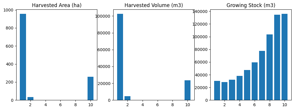
Now we can run our model again with run_scenario, passing in the new harvest volume flow constraint parameters.

run_scenario(fm, "scenario-3", ws3.opt.SENSE_MAXIMIZE, acodes, coeff_funcs, cflw_e, cgen_data)

(<Figure size 1200x400 with 3 Axes>,
    period        oha           ohv            ogs
 0       1  81.490393  11505.674653  137557.296765
 1       2  88.328985  12080.958385  136215.193742
 2       3  75.802288  12080.958385  133278.227164
 3       4  79.588800  10930.390920  132205.401813
 4       5  79.657228  10930.390920  133028.457906
 5       6  79.744249  10930.390920  134576.453980
 6       7  80.687348  10930.390920  136326.683219
 7       8  79.987614  10930.390920  137283.043147
 8       9  79.434817  10930.390920  137053.561019
 9      10  68.242127  10930.390920  135984.046132,
 <ws3.opt.Problem at 0x74e89027cf80>)

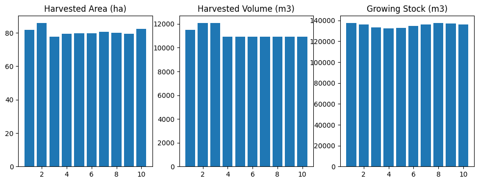
Ta da! That is starting to look more like a sustainable harvesting solution. The combination of ending inventory constraint and even-flow harest volume constraint is effectively stabilizing both log production and growing stock inventory. There is a bit of a spike in the harvested area in the final time step, though, which we can try to mitigate by adding a flow constraint on harvest area (we will leave all the previously defined constraints in the model, including the harvest volume flow constraint we added in the previous step).

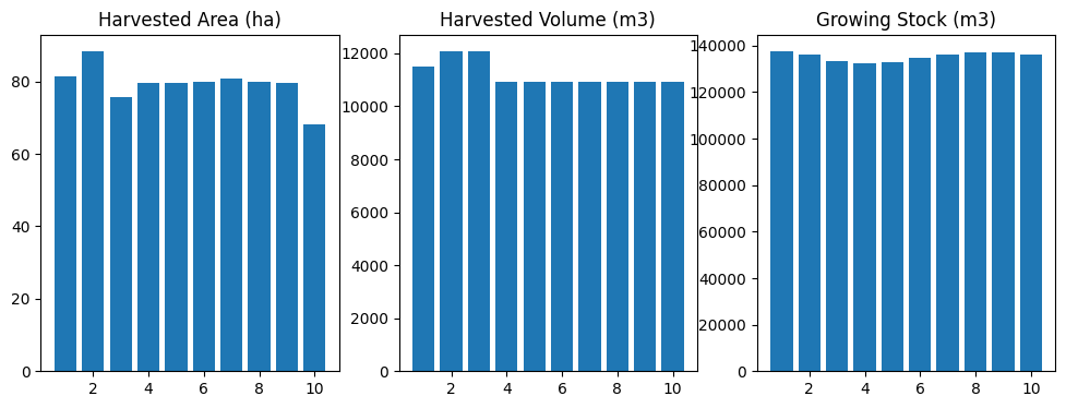
4.5.3.4. Adding harvest area even-flow constraints

We can use the same cmp_c_caa coefficient function that we used above to define the harvest volume flow constraint, but just use a different value for the expr arg (1. instead of totvol * 0.85) in the call to functools.partial. We will use the same espilon value of 0.05 that we used above to define the harvest volume flow constraint.

coeff_funcs["cflw_ha"] = functools.partial(cmp_c_caa, expr="1.", acodes=["harvest"])
cflw_e["cflw_ha"] = ({p:0.05 for p in fm.periods}, 1)

fig, df, p = run_scenario(fm, "scenario-4", ws3.opt.SENSE_MAXIMIZE, acodes, coeff_funcs, cflw_e, cgen_data)

Looking good! That spike in harvest area in period 10 is gone, but everything else still looks OK. This illustrates a typical approach that professional analysts would use to to add new constraints and re-run the model.

We will now use this approach to add a constraint that forces harvest area in period 1 to be a maximum of 40 hectares to simulate a “what if” question approach to forest resource analysis (in this case asking the question, “What if we capped harvest volume to about half the maximum sustainable harvest rate?”). Note that in a realistic analysis that uses the optimization modelling functions, you do not need to include all the performance indicators you want to track in the model in the optimization model. You can limit optimization model indicators to the indicators that you need to define the objective function and constraints, and then define and compile any number of additional performance indicators that you apply to your ws3 simulation in a post hoc analysis phase (after solving the optimization model and running the simulation in ws3).

Before running the next iteration of our model in the next section, we will calculate the mean yield (\(m^3/ha\)) for the last scenario we ran so we can observe the impact of reducing harvest level on yield.

df_yield_1 = df["ohv"] / df["oha"]
df_yield_1

0    140.587682
1    140.587682
2    155.386386
3    137.338148
4    137.220378
5    137.075846
6    135.471071
7    136.652859
8    137.604713
9    132.681064
dtype: float64

4.5.3.5. Adding an upper bound constraint on period-1 harvest area

Now that we are on a roll and have everything all set up to update and re-run the model with a few lines of code, we can add an upper bound constraint on period 1 harvest area (maximum 40 hectares, about half the area harvested in the current solution). Even though we only constrain period 1 harvest area, the harvest area flow constraints should force a reduced harvest area in all other periods as well.

coeff_funcs["cgen_ha"] = functools.partial(cmp_c_caa, expr="1.", acodes=["harvest"])
cgen_data["cgen_ha"] = {"lb":{1:0.}, "ub":{1:40.}}

fig, df, p = run_scenario(fm, "scenario-5", ws3.opt.SENSE_MAXIMIZE, acodes, coeff_funcs, cflw_e, cgen_data)

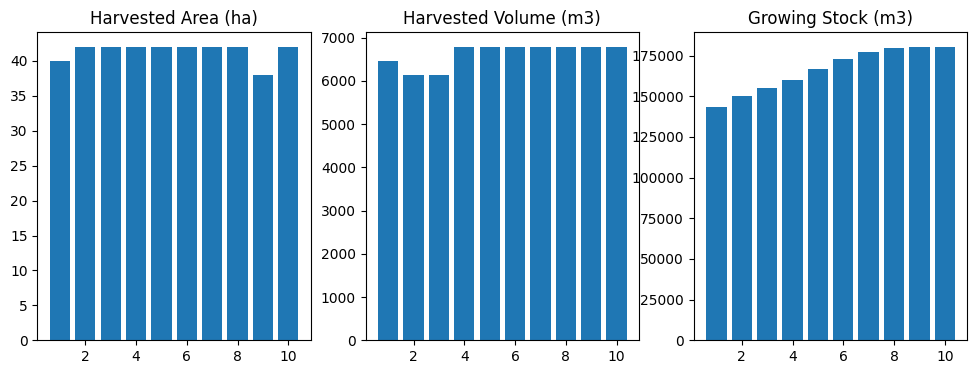
As expected, harvest area is down to about 40 hectares per period (and respecting even flow constraints). Not surprisingly (if you understand how forests work), this induced a similar reduction in the harvest area. Also not surprisingly, harvesting fewer trees each year results in an accumulation of growing stock in the forest (compare with the previous scenarios, where the growsing stock inventory was relatively constant throughout the simulation horizon).

Now lets recalculate our mean yield metric.

df_yield_2 = df["ohv"] / df["oha"]
df_yield_2

0    161.535231
1    146.150923
2    146.150923
3    161.535231
4    161.535231
5    161.535231
6    161.535231
7    161.535231
8    178.538939
9    161.535231
dtype: float64

Now lets calculate some statistics comparing these yield results from the last two scenarios we ran.

df_diff_abs = df_yield_2 - df_yield_1
df_diff_rel = (df_diff_abs / df_yield_1) * 100.
df_diff_abs, df_diff_rel, df_diff_abs.mean(), df_diff_rel.mean()

(0    20.947548
 1     5.563241
 2    -9.235463
 3    24.197082
 4    24.314853
 5    24.459385
 6    26.064160
 7    24.882371
 8    40.934226
 9    28.854167
 dtype: float64,
 0    14.899988
 1     3.957132
 2    -5.943547
 3    17.618617
 4    17.719564
 5    17.843687
 6    19.239650
 7    18.208453
 8    29.747692
 9    21.747012
 dtype: float64,
 np.float64(21.098157013702718),
 np.float64(15.503824824706948))

So on average yield is 21 \(m^3/ha\) (16%) more in the reduced harvest scenario compared to the refernece scenario. This is not surprising as reducing even-flow harvest level will tend to lengthen rotation length, so stands have time to accumulate more merchantable yield (trees grow larger if given more time!) before they get harvested.

4.5.3.6. Defining an infeasible optimization model

Next, we deliberately define an infeasible pair of constraintints on the harvest area. This is done by setting the lower bound of the harvest area constraint to be 50 hectares per period and the upper bound to 40 hectares per period (which is obviously mathematically impossible).

cgen_data["cgen_ha"] = {"lb":{1:50.}, "ub":{1:40.}}
run_scenario(fm, "scenario-6", ws3.opt.SENSE_MAXIMIZE, acodes, coeff_funcs, cflw_e, cgen_data, verbose=True)

add_problem: build problem
generate trees using 1 workers
process trees
_bld_p_m1: build problem
_bld_p_m1: done building problem
add_problem: compile flow constraints
_cmp_cflw_m1: phase 1
_cmp_cflw_m1: phase 2
_cmp_cflw_m1: phase 3
add_problem: compile general constraints
Running HiGHS 1.11.0 (git hash: 364c83a): Copyright (c) 2025 HiGHS under MIT licence terms
LP   has 76 rows; 305 cols; 3813 nonzeros
Coefficient ranges:
  Matrix [3e-02, 5e+04]
  Cost   [2e+01, 4e+04]
  Bound  [1e+00, 1e+00]
  RHS    [1e+00, 1e+09]
Presolving model
63 rows, 297 cols, 3441 nonzeros  0s
Model not optimal.
Problem status detected on presolve: Infeasible
Model status        : Infeasible
Objective value     :  0.0000000000e+00
HiGHS run time      :          0.00

(None, None, <ws3.opt.Problem at 0x74e8c0372ae0>)

Our run_scenario function does not have very advanced error handling implemented, but you can still see from the solver output that the problem in infeasible (so no solution compiled or displayed for this case).

You would not typically deliberately define an infeasible constraint, but it is a good exercise to do so just to make sure you understand what infeasible solutions are (and how you end up with one).