4.8. Spatially allocating a ws3 harvest schedule to raster grids

This tutorial demonstrates how to take an aspatial harvest schedule produced by ws3, disaggregate it to annual steps, and allocate it across a rasterized forest inventory using the `ws3.spatial.ForestRaster <https://ws3.readthedocs.io/en/latest/api.html#ws3.spatial.ForestRaster>`__ class. The workflow mirrors the spatial allocation utilities used by spades_ws3, but keeps things self-contained inside this repository.

We will:

• build a ForestModel from the sample Woodstock-format files

• generate a quick heuristic harvest schedule

• rasterize the sample stand inventory shapefile to a three-band GeoTIFF (hash, age, block id)

• use ForestRaster to convert the 10-year schedule into annual GeoTIFF disturbance maps

• inspect the resulting rasters and summarise disturbed area per year

4.8.1. Recommended environment

As with the other notebooks in this folder, running inside a sandboxed virtual environment keeps dependencies tidy (see 000_venv_python_kernel_setup.ipynb). The commands below assume this notebook lives inside the WS3 repository checkout.

%load_ext autoreload
%autoreload 2

clobber_ws3 = False
if clobber_ws3:
    %pip uninstall -y ws3
    %pip install -e ..

import sys
from pathlib import Path
import numpy as np
import pandas as pd
import rasterio
import matplotlib.pyplot as plt

# allow notebooks to reuse helper utilities in this folder
EXAMPLES_DIR = Path.cwd() / 'examples'
if str(EXAMPLES_DIR) not in sys.path:
    sys.path.insert(0, str(EXAMPLES_DIR))

import ws3.forest
from ws3.common import rasterize_stands, hash_dt
from ws3.spatial import ForestRaster
from util import schedule_harvest_areacontrol, compile_scenario, plot_scenario

4.8.2. Data paths

We re-use the sample TSA 24 dataset bundled with the repository. The Woodstock formatted files feed the forest model, while the companion shapefile provides a spatial inventory for rasterization.

#DATA_DIR = Path('examples/data')
DATA_DIR = Path('data')
WOODSTOCK_DIR = DATA_DIR / 'woodstock_model_files_tsa24_clipped'
SHAPE_PATH = DATA_DIR / 'shp' / 'tsa24_clipped.shp' / 'stands.shp'

# output directories (created on demand)
RASTER_DIR = DATA_DIR / 'raster_spatial_demo'
RASTER_DIR.mkdir(parents=True, exist_ok=True)
INVENTORY_TIF = RASTER_DIR / 'tsa24_inventory.tif'

SPATIAL_DIR = DATA_DIR / 'spatial_outputs' / 'tsa24_demo'
SPATIAL_DIR.mkdir(parents=True, exist_ok=True)

INVENTORY_TIF, SPATIAL_DIR

(PosixPath('data/raster_spatial_demo/tsa24_inventory.tif'),
 PosixPath('data/spatial_outputs/tsa24_demo'))

4.8.3. Build a ForestModel

We load the Woodstock-format inputs, initialise state, and keep the horizon short (5 periods of 10 years) so that the spatial allocation step produces a manageable number of rasters.

BASE_YEAR = 2020
HORIZON = 5
PERIOD_LENGTH = 10

fm = ws3.forest.ForestModel(
    model_name='tsa24_clipped',
    model_path=str(WOODSTOCK_DIR),
    base_year=BASE_YEAR,
    horizon=HORIZON,
    period_length=PERIOD_LENGTH,
    max_age=1000,
)

fm.import_landscape_section()
fm.import_areas_section(convert_periods_to_years=period_length)
fm.import_yields_section(convert_periods_to_years=period_length)
fm.import_actions_section(convert_periods_to_years=period_length)
fm.import_transitions_section(convert_periods_to_years=period_length)
fm.initialize_areas()
fm.add_null_action()
fm.reset_actions()

fm

<ws3.forest.ForestModel at 0x7a02b8306de0>

4.8.4. Heuristic harvest schedule

We call the schedule_harvest_areacontrol helper (defined in examples/util.py) to generate an aspatial schedule. The function compiles the internal applied_actions structure, which ForestRaster will later consume.

sch = schedule_harvest_areacontrol(fm)
scenario = compile_scenario(fm)
scenario

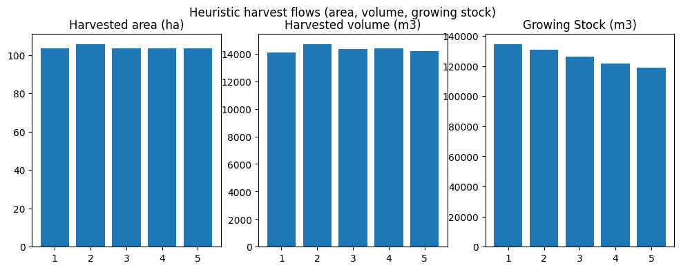
	period	oha	ohv	ogs
0	1	103.411088	14069.080670	134541.524980
1	2	105.655079	14690.387934	130879.310887
2	3	103.411088	14352.583697	126127.588834
3	4	103.411088	14403.805319	121730.561271
4	5	103.411088	14167.526587	119035.437396

fig, axes = plot_scenario(scenario)
fig.suptitle('Heuristic harvest flows (area, volume, growing stock)')
plt.show()

4.8.4.1. Ensure transition lookups cover scheduled ages

Some Woodstock models only declare a generic transition for age = -1. The snippet below mirrors what spades_ws3 does: it copies those generic transitions to every (action, age) pair actually referenced in the schedule, so that ForestRaster can resolve targets without raising a KeyError.

for period in fm.periods:
    for acode, by_dtype in fm.applied_actions[period].items():
        for dtk, by_age in by_dtype.items():
            dt = fm.dtypes[dtk]
            for age in list(by_age.keys()):
                if (acode, age) not in dt.transitions:
                    if (acode, -1) in dt.transitions:
                        dt.transitions[acode, age] = dt.transitions[acode, -1]
                    else:
                        raise KeyError(f"Missing transition for {(acode, age)} in {dtk}")

4.8.5. Rasterize the stand inventory

ForestRaster expects a three-band raster: band 1 stores hashed development type theme values, band 2 stores age (years), and band 3 stores block IDs. The helper ws3.common.rasterize_stands creates this raster from the sample shapefile and returns the required hash map.

theme_columns = ['theme0', 'theme1', 'theme2', 'theme3', 'curve1']

hdt_map = rasterize_stands(
    str(SHAPE_PATH),
    str(INVENTORY_TIF),
    theme_cols=theme_columns,
    age_col='age',
    blk_col='curve2',
    age_divisor=1.0,
)

with rasterio.open(INVENTORY_TIF) as src:
    print('Raster shape:', src.count, 'bands', src.width, 'x', src.height)
    print('CRS:', src.crs)
    print('Pixel size:', src.transform.a, 'm')
    print('Hash map entries:', len(hdt_map))

Raster shape: 3 bands 41 x 41
CRS: EPSG:3005
Pixel size: 100.0 m
Hash map entries: 12

4.8.6. Allocate the schedule to rasters

We instantiate ForestRaster with the model, hash metadata, and destination directory. The planner horizon of five periods (10-year periods) becomes 50 annual GeoTIFFs. Each file encodes whether a cell is disturbed (1) or untouched (nodata/0) for the target year.

# clean older outputs from previous runs
for tif in SPATIAL_DIR.glob('harvested_*.tif'):
    tif.unlink()

forest_raster = ForestRaster(
    hdt_map=hdt_map,
    hdt_func=hash_dt,
    src_path=str(INVENTORY_TIF),
    snk_path=str(SPATIAL_DIR),
    acode_map={'harvest': 'harvested'},
    forestmodel=fm,
    base_year=BASE_YEAR,
    horizon=HORIZON,
    period_length=PERIOD_LENGTH,
    time_step=1,
    piggyback_acodes={},
)

forest_raster.allocate_schedule(verbose=False, sda_mode='randblk', nthresh=10)
forest_raster.cleanup()

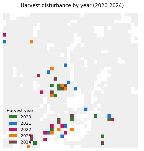
4.8.7. Inspect the outputs

The allocation step writes one GeoTIFF per year. Below we list the first few files, visualise the first raster, and summarise the disturbed area (in number of pixels) per year.

output_files = sorted(SPATIAL_DIR.glob('harvested_*.tif'))
output_files[:5]

[PosixPath('data/spatial_outputs/tsa24_demo/harvested_2020.tif'),
 PosixPath('data/spatial_outputs/tsa24_demo/harvested_2021.tif'),
 PosixPath('data/spatial_outputs/tsa24_demo/harvested_2022.tif'),
 PosixPath('data/spatial_outputs/tsa24_demo/harvested_2023.tif'),
 PosixPath('data/spatial_outputs/tsa24_demo/harvested_2024.tif')]

years_to_display = [BASE_YEAR + i for i in range(5)]
files_by_year = {int(path.stem.split('_')[1]): path for path in output_files}
available = [(year, files_by_year[year]) for year in years_to_display if year in files_by_year]

if not available:
    raise ValueError('No harvest rasters found for the requested years.')

from matplotlib.colors import ListedColormap, BoundaryNorm
from matplotlib.patches import Patch

with rasterio.open(INVENTORY_TIF) as src:
    inventory = src.read(1)
    inv_nodata = src.nodata
    template_shape = inventory.shape
    if inv_nodata is None:
        forest_mask = np.ma.array(np.ones(template_shape, dtype=int), mask=np.isnan(inventory))
    else:
        forest_mask = np.ma.array(np.ones(template_shape, dtype=int), mask=(inventory == inv_nodata))

display = np.full(template_shape, fill_value=-1, dtype=int)

for idx, (year, tif_path) in enumerate(available):
    with rasterio.open(tif_path) as src:
        arr = src.read(1)
        nodata = src.nodata
        if nodata is None:
            harvested = ~np.isnan(arr)
        else:
            harvested = arr != nodata
        display = np.where(harvested, idx, display)

masked_display = np.ma.array(display, mask=display == -1)

color_palette = ['#2E7D32', '#1976D2', '#C2185B', '#F57C00', '#6D4C41'][:len(available)]
harvest_cmap = ListedColormap(color_palette)
norm = BoundaryNorm(range(len(color_palette) + 1), harvest_cmap.N)
background_cmap = ListedColormap(['#e0e0e0'])

fig, ax = plt.subplots(figsize=(6, 6))
ax.imshow(forest_mask, cmap=background_cmap, interpolation='nearest', alpha=0.5)
ax.imshow(masked_display, cmap=harvest_cmap, norm=norm, interpolation='nearest')
ax.set_title(f"Harvest disturbance by year ({available[0][0]}-{available[-1][0]})")
ax.axis('off')

handles = [Patch(facecolor=color_palette[i], label=str(year)) for i, (year, _) in enumerate(available)]
ax.legend(handles=handles, title='Harvest year', loc='lower left', frameon=False)
plt.show()

summary = []
for tif in output_files:
    year = int(tif.stem.split('_')[1])
    with rasterio.open(tif) as src:
        arr = src.read(1)
        nodata = src.nodata
        disturbed = np.count_nonzero(arr != nodata)
    summary.append({'year': year, 'disturbed_pixels': disturbed})

pd.DataFrame(summary).head()

	year	disturbed_pixels
0	2020	10
1	2021	10
2	2022	10
3	2023	9
4	2024	9

4.8.7.1. Next steps

• Supply your own management-unit mask by passing a tuple (e.g., ('tsa24_clipped', '1', '?', '?', '?')) to ForestRaster.allocate_schedule.

• Use finer time steps (e.g., quarterly) by setting time_step=0.25 when building ForestRaster.

• Combine multiple actions by expanding acode_map (each entry gets its own set of year-indexed rasters).

Remember to tidy up raster outputs if the directory should remain clean for version control.