4.11. Implement the Neilson hack using ws3 and libcbm (from scratch)
In this notebook we show how to implement the Neilson hack (i.e., generate carbon yield curves from a CBM for use in a forest estate model) using ws3 and libcbm.
In a nutshell, the Neilson hack consists of running a CBM from forest estate model output (see example notebook 030 and 031 for details), except that the inventory table gets hacked to have one record per development type (with age set to 0 and area set to 1) and no disturabance events are simulated. Carbon stock and flux data exported from the CBM can then be reformatted and imported in the forest estate model as carbon yield curves. That is about it. Should work for just about any ws3
model. See Neilson et al. (2006) for details.
Neilson, E. T., MacLean, D. A., Arp, P. A., Meng, F. R., Bourque, C. P., & Bhatti, J. S. (2006). Modeling carbon sequestration with CO2Fix and a timber supply model for use in forest management planning. Canadian journal of soil science, 86(Special Issue), 219-233.
In this notebook, we implement the Neilson hack from scratch. In notebook 041 we show how to use built-in ws3 functions to automate this.
4.11.1. Set up modelling environment
First, make sure we have the correct versions of ws3 and libcbm installed. Both of these packages are relatively new and under active development, it is best we stick to known-working versions of each package from their respective GitHub repos.
We strongly recommend that you run this notebook in venv-sandboxed Python kernel (see
venv_python_kernel_setupnotebook for an example of how to do this). This will ensure that you are working from a fresh Python package environment, and not wasting time debugging random interactions between this notebook and whatever mishmash of packages you have installed on your system in various parts of your Python path. You have been warned.
[1]:
%load_ext autoreload
%autoreload 2
Optionally, uninstall the ws3 package and replace it with a pointer to this local clone of the GitHub repository code (useful if you want ot tweak the source code for whatever reason).
[2]:
clobber_ws3 = True
if clobber_ws3:
    %pip uninstall -y ws3
    %pip install -e ..
Found existing installation: ws3 1.1.0.dev0
Uninstalling ws3-1.1.0.dev0:
  Successfully uninstalled ws3-1.1.0.dev0
Note: you may need to restart the kernel to use updated packages.
Obtaining file:///home/gep/tmp/ws3
  Installing build dependencies ... done
  Checking if build backend supports build_editable ... done
  Getting requirements to build editable ... done
  Installing backend dependencies ... done
  Preparing editable metadata (pyproject.toml) ... done
Requirement already satisfied: dill in /home/gep/tmp/ws3/.venv/lib/python3.12/site-packages (from ws3==1.1.0.dev0) (0.4.0)
Requirement already satisfied: fiona in /home/gep/tmp/ws3/.venv/lib/python3.12/site-packages (from ws3==1.1.0.dev0) (1.10.1)
Requirement already satisfied: gurobipy in /home/gep/tmp/ws3/.venv/lib/python3.12/site-packages (from ws3==1.1.0.dev0) (12.0.3)
Requirement already satisfied: highspy in /home/gep/tmp/ws3/.venv/lib/python3.12/site-packages (from ws3==1.1.0.dev0) (1.11.0)
Requirement already satisfied: libcbm in /home/gep/tmp/ws3/.venv/lib/python3.12/site-packages (from ws3==1.1.0.dev0) (2.8.1)
Requirement already satisfied: matplotlib in /home/gep/tmp/ws3/.venv/lib/python3.12/site-packages (from ws3==1.1.0.dev0) (3.10.5)
Requirement already satisfied: numpy>=1.21 in /home/gep/tmp/ws3/.venv/lib/python3.12/site-packages (from ws3==1.1.0.dev0) (2.2.6)
Requirement already satisfied: pandas>=1.3 in /home/gep/tmp/ws3/.venv/lib/python3.12/site-packages (from ws3==1.1.0.dev0) (2.3.1)
Requirement already satisfied: profilehooks in /home/gep/tmp/ws3/.venv/lib/python3.12/site-packages (from ws3==1.1.0.dev0) (1.13.0)
Requirement already satisfied: pulp in /home/gep/tmp/ws3/.venv/lib/python3.12/site-packages (from ws3==1.1.0.dev0) (3.2.2)
Requirement already satisfied: rasterio in /home/gep/tmp/ws3/.venv/lib/python3.12/site-packages (from ws3==1.1.0.dev0) (1.4.3)
Requirement already satisfied: scipy>=1.7 in /home/gep/tmp/ws3/.venv/lib/python3.12/site-packages (from ws3==1.1.0.dev0) (1.16.1)
Requirement already satisfied: python-dateutil>=2.8.2 in /home/gep/tmp/ws3/.venv/lib/python3.12/site-packages (from pandas>=1.3->ws3==1.1.0.dev0) (2.9.0.post0)
Requirement already satisfied: pytz>=2020.1 in /home/gep/tmp/ws3/.venv/lib/python3.12/site-packages (from pandas>=1.3->ws3==1.1.0.dev0) (2025.2)
Requirement already satisfied: tzdata>=2022.7 in /home/gep/tmp/ws3/.venv/lib/python3.12/site-packages (from pandas>=1.3->ws3==1.1.0.dev0) (2025.2)
Requirement already satisfied: six>=1.5 in /home/gep/tmp/ws3/.venv/lib/python3.12/site-packages (from python-dateutil>=2.8.2->pandas>=1.3->ws3==1.1.0.dev0) (1.17.0)
Requirement already satisfied: attrs>=19.2.0 in /home/gep/tmp/ws3/.venv/lib/python3.12/site-packages (from fiona->ws3==1.1.0.dev0) (25.3.0)
Requirement already satisfied: certifi in /home/gep/tmp/ws3/.venv/lib/python3.12/site-packages (from fiona->ws3==1.1.0.dev0) (2025.8.3)
Requirement already satisfied: click~=8.0 in /home/gep/tmp/ws3/.venv/lib/python3.12/site-packages (from fiona->ws3==1.1.0.dev0) (8.2.1)
Requirement already satisfied: click-plugins>=1.0 in /home/gep/tmp/ws3/.venv/lib/python3.12/site-packages (from fiona->ws3==1.1.0.dev0) (1.1.1.2)
Requirement already satisfied: cligj>=0.5 in /home/gep/tmp/ws3/.venv/lib/python3.12/site-packages (from fiona->ws3==1.1.0.dev0) (0.7.2)
Requirement already satisfied: numexpr>=2.8.7 in /home/gep/tmp/ws3/.venv/lib/python3.12/site-packages (from libcbm->ws3==1.1.0.dev0) (2.11.0)
Requirement already satisfied: numba in /home/gep/tmp/ws3/.venv/lib/python3.12/site-packages (from libcbm->ws3==1.1.0.dev0) (0.61.2)
Requirement already satisfied: pyyaml in /home/gep/tmp/ws3/.venv/lib/python3.12/site-packages (from libcbm->ws3==1.1.0.dev0) (6.0.2)
Requirement already satisfied: mock in /home/gep/tmp/ws3/.venv/lib/python3.12/site-packages (from libcbm->ws3==1.1.0.dev0) (5.2.0)
Requirement already satisfied: openpyxl in /home/gep/tmp/ws3/.venv/lib/python3.12/site-packages (from libcbm->ws3==1.1.0.dev0) (3.1.5)
Requirement already satisfied: contourpy>=1.0.1 in /home/gep/tmp/ws3/.venv/lib/python3.12/site-packages (from matplotlib->ws3==1.1.0.dev0) (1.3.3)
Requirement already satisfied: cycler>=0.10 in /home/gep/tmp/ws3/.venv/lib/python3.12/site-packages (from matplotlib->ws3==1.1.0.dev0) (0.12.1)
Requirement already satisfied: fonttools>=4.22.0 in /home/gep/tmp/ws3/.venv/lib/python3.12/site-packages (from matplotlib->ws3==1.1.0.dev0) (4.59.0)
Requirement already satisfied: kiwisolver>=1.3.1 in /home/gep/tmp/ws3/.venv/lib/python3.12/site-packages (from matplotlib->ws3==1.1.0.dev0) (1.4.8)
Requirement already satisfied: packaging>=20.0 in /home/gep/tmp/ws3/.venv/lib/python3.12/site-packages (from matplotlib->ws3==1.1.0.dev0) (25.0)
Requirement already satisfied: pillow>=8 in /home/gep/tmp/ws3/.venv/lib/python3.12/site-packages (from matplotlib->ws3==1.1.0.dev0) (11.3.0)
Requirement already satisfied: pyparsing>=2.3.1 in /home/gep/tmp/ws3/.venv/lib/python3.12/site-packages (from matplotlib->ws3==1.1.0.dev0) (3.2.3)
Requirement already satisfied: llvmlite<0.45,>=0.44.0dev0 in /home/gep/tmp/ws3/.venv/lib/python3.12/site-packages (from numba->libcbm->ws3==1.1.0.dev0) (0.44.0)
Requirement already satisfied: et-xmlfile in /home/gep/tmp/ws3/.venv/lib/python3.12/site-packages (from openpyxl->libcbm->ws3==1.1.0.dev0) (2.0.0)
Requirement already satisfied: affine in /home/gep/tmp/ws3/.venv/lib/python3.12/site-packages (from rasterio->ws3==1.1.0.dev0) (2.4.0)
Building wheels for collected packages: ws3
  Building editable for ws3 (pyproject.toml) ... done
  Created wheel for ws3: filename=ws3-1.1.0.dev0-py3-none-any.whl size=4136 sha256=5df49d1809d2f15004f3046010971c142390fb47fb3bfa7620b09e11903424a7
  Stored in directory: /tmp/pip-ephem-wheel-cache-gqh8kf6a/wheels/fa/4b/10/3fe4b92a02fb87987a6fe53a10fad0a22a781bf98cd7b63f17
Successfully built ws3
Installing collected packages: ws3
Successfully installed ws3-1.1.0.dev0
Note: you may need to restart the kernel to use updated packages.
Use pip to install Python packages listed in requirements.txt (some extra packages needed for example notebooks to run correctly).
[3]:
%pip install -r requirements.txt
Requirement already satisfied: seaborn in /home/gep/tmp/ws3/.venv/lib/python3.12/site-packages (from -r requirements.txt (line 1)) (0.13.2)
Requirement already satisfied: geopandas in /home/gep/tmp/ws3/.venv/lib/python3.12/site-packages (from -r requirements.txt (line 2)) (1.1.1)
Requirement already satisfied: ipywidgets in /home/gep/tmp/ws3/.venv/lib/python3.12/site-packages (from -r requirements.txt (line 3)) (8.1.7)
Requirement already satisfied: numpy!=1.24.0,>=1.20 in /home/gep/tmp/ws3/.venv/lib/python3.12/site-packages (from seaborn->-r requirements.txt (line 1)) (2.2.6)
Requirement already satisfied: pandas>=1.2 in /home/gep/tmp/ws3/.venv/lib/python3.12/site-packages (from seaborn->-r requirements.txt (line 1)) (2.3.1)
Requirement already satisfied: matplotlib!=3.6.1,>=3.4 in /home/gep/tmp/ws3/.venv/lib/python3.12/site-packages (from seaborn->-r requirements.txt (line 1)) (3.10.5)
Requirement already satisfied: pyogrio>=0.7.2 in /home/gep/tmp/ws3/.venv/lib/python3.12/site-packages (from geopandas->-r requirements.txt (line 2)) (0.11.1)
Requirement already satisfied: packaging in /home/gep/tmp/ws3/.venv/lib/python3.12/site-packages (from geopandas->-r requirements.txt (line 2)) (25.0)
Requirement already satisfied: pyproj>=3.5.0 in /home/gep/tmp/ws3/.venv/lib/python3.12/site-packages (from geopandas->-r requirements.txt (line 2)) (3.7.1)
Requirement already satisfied: shapely>=2.0.0 in /home/gep/tmp/ws3/.venv/lib/python3.12/site-packages (from geopandas->-r requirements.txt (line 2)) (2.1.1)
Requirement already satisfied: comm>=0.1.3 in /home/gep/tmp/ws3/.venv/lib/python3.12/site-packages (from ipywidgets->-r requirements.txt (line 3)) (0.2.3)
Requirement already satisfied: ipython>=6.1.0 in /home/gep/tmp/ws3/.venv/lib/python3.12/site-packages (from ipywidgets->-r requirements.txt (line 3)) (9.4.0)
Requirement already satisfied: traitlets>=4.3.1 in /home/gep/tmp/ws3/.venv/lib/python3.12/site-packages (from ipywidgets->-r requirements.txt (line 3)) (5.14.3)
Requirement already satisfied: widgetsnbextension~=4.0.14 in /home/gep/tmp/ws3/.venv/lib/python3.12/site-packages (from ipywidgets->-r requirements.txt (line 3)) (4.0.14)
Requirement already satisfied: jupyterlab_widgets~=3.0.15 in /home/gep/tmp/ws3/.venv/lib/python3.12/site-packages (from ipywidgets->-r requirements.txt (line 3)) (3.0.15)
Requirement already satisfied: decorator in /home/gep/tmp/ws3/.venv/lib/python3.12/site-packages (from ipython>=6.1.0->ipywidgets->-r requirements.txt (line 3)) (5.2.1)
Requirement already satisfied: ipython-pygments-lexers in /home/gep/tmp/ws3/.venv/lib/python3.12/site-packages (from ipython>=6.1.0->ipywidgets->-r requirements.txt (line 3)) (1.1.1)
Requirement already satisfied: jedi>=0.16 in /home/gep/tmp/ws3/.venv/lib/python3.12/site-packages (from ipython>=6.1.0->ipywidgets->-r requirements.txt (line 3)) (0.19.2)
Requirement already satisfied: matplotlib-inline in /home/gep/tmp/ws3/.venv/lib/python3.12/site-packages (from ipython>=6.1.0->ipywidgets->-r requirements.txt (line 3)) (0.1.7)
Requirement already satisfied: pexpect>4.3 in /home/gep/tmp/ws3/.venv/lib/python3.12/site-packages (from ipython>=6.1.0->ipywidgets->-r requirements.txt (line 3)) (4.9.0)
Requirement already satisfied: prompt_toolkit<3.1.0,>=3.0.41 in /home/gep/tmp/ws3/.venv/lib/python3.12/site-packages (from ipython>=6.1.0->ipywidgets->-r requirements.txt (line 3)) (3.0.51)
Requirement already satisfied: pygments>=2.4.0 in /home/gep/tmp/ws3/.venv/lib/python3.12/site-packages (from ipython>=6.1.0->ipywidgets->-r requirements.txt (line 3)) (2.19.2)
Requirement already satisfied: stack_data in /home/gep/tmp/ws3/.venv/lib/python3.12/site-packages (from ipython>=6.1.0->ipywidgets->-r requirements.txt (line 3)) (0.6.3)
Requirement already satisfied: wcwidth in /home/gep/tmp/ws3/.venv/lib/python3.12/site-packages (from prompt_toolkit<3.1.0,>=3.0.41->ipython>=6.1.0->ipywidgets->-r requirements.txt (line 3)) (0.2.13)
Requirement already satisfied: parso<0.9.0,>=0.8.4 in /home/gep/tmp/ws3/.venv/lib/python3.12/site-packages (from jedi>=0.16->ipython>=6.1.0->ipywidgets->-r requirements.txt (line 3)) (0.8.4)
Requirement already satisfied: contourpy>=1.0.1 in /home/gep/tmp/ws3/.venv/lib/python3.12/site-packages (from matplotlib!=3.6.1,>=3.4->seaborn->-r requirements.txt (line 1)) (1.3.3)
Requirement already satisfied: cycler>=0.10 in /home/gep/tmp/ws3/.venv/lib/python3.12/site-packages (from matplotlib!=3.6.1,>=3.4->seaborn->-r requirements.txt (line 1)) (0.12.1)
Requirement already satisfied: fonttools>=4.22.0 in /home/gep/tmp/ws3/.venv/lib/python3.12/site-packages (from matplotlib!=3.6.1,>=3.4->seaborn->-r requirements.txt (line 1)) (4.59.0)
Requirement already satisfied: kiwisolver>=1.3.1 in /home/gep/tmp/ws3/.venv/lib/python3.12/site-packages (from matplotlib!=3.6.1,>=3.4->seaborn->-r requirements.txt (line 1)) (1.4.8)
Requirement already satisfied: pillow>=8 in /home/gep/tmp/ws3/.venv/lib/python3.12/site-packages (from matplotlib!=3.6.1,>=3.4->seaborn->-r requirements.txt (line 1)) (11.3.0)
Requirement already satisfied: pyparsing>=2.3.1 in /home/gep/tmp/ws3/.venv/lib/python3.12/site-packages (from matplotlib!=3.6.1,>=3.4->seaborn->-r requirements.txt (line 1)) (3.2.3)
Requirement already satisfied: python-dateutil>=2.7 in /home/gep/tmp/ws3/.venv/lib/python3.12/site-packages (from matplotlib!=3.6.1,>=3.4->seaborn->-r requirements.txt (line 1)) (2.9.0.post0)
Requirement already satisfied: pytz>=2020.1 in /home/gep/tmp/ws3/.venv/lib/python3.12/site-packages (from pandas>=1.2->seaborn->-r requirements.txt (line 1)) (2025.2)
Requirement already satisfied: tzdata>=2022.7 in /home/gep/tmp/ws3/.venv/lib/python3.12/site-packages (from pandas>=1.2->seaborn->-r requirements.txt (line 1)) (2025.2)
Requirement already satisfied: ptyprocess>=0.5 in /home/gep/tmp/ws3/.venv/lib/python3.12/site-packages (from pexpect>4.3->ipython>=6.1.0->ipywidgets->-r requirements.txt (line 3)) (0.7.0)
Requirement already satisfied: certifi in /home/gep/tmp/ws3/.venv/lib/python3.12/site-packages (from pyogrio>=0.7.2->geopandas->-r requirements.txt (line 2)) (2025.8.3)
Requirement already satisfied: six>=1.5 in /home/gep/tmp/ws3/.venv/lib/python3.12/site-packages (from python-dateutil>=2.7->matplotlib!=3.6.1,>=3.4->seaborn->-r requirements.txt (line 1)) (1.17.0)
Requirement already satisfied: executing>=1.2.0 in /home/gep/tmp/ws3/.venv/lib/python3.12/site-packages (from stack_data->ipython>=6.1.0->ipywidgets->-r requirements.txt (line 3)) (2.2.0)
Requirement already satisfied: asttokens>=2.1.0 in /home/gep/tmp/ws3/.venv/lib/python3.12/site-packages (from stack_data->ipython>=6.1.0->ipywidgets->-r requirements.txt (line 3)) (3.0.0)
Requirement already satisfied: pure-eval in /home/gep/tmp/ws3/.venv/lib/python3.12/site-packages (from stack_data->ipython>=6.1.0->ipywidgets->-r requirements.txt (line 3)) (0.2.3)
Note: you may need to restart the kernel to use updated packages.
Create a ForestModel instance by loading Woodstock-formatted input files.
[4]:
import ws3.forest
[5]:
base_year = 2020
horizon = 10
period_length = 10
max_age = 1000
tvy_name = "totvol"
[6]:
fm = ws3.forest.ForestModel(model_name="tsa24_clipped",
                            model_path="data/woodstock_model_files_tsa24_clipped",
                            base_year=base_year,
                            horizon=horizon,
                            period_length=period_length,
                            max_age=max_age)
fm.import_landscape_section()
fm.import_areas_section(convert_periods_to_years=period_length)
fm.import_yields_section(convert_periods_to_years=period_length)
fm.import_actions_section(convert_periods_to_years=period_length)
fm.import_transitions_section(convert_periods_to_years=period_length)
fm.initialize_areas()
fm.add_null_action()
fm.reset_actions()
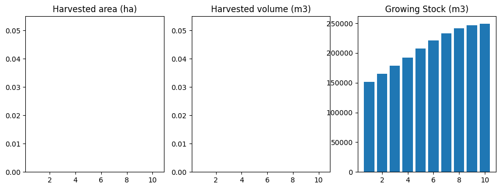
Schedule some harvesting in our ws3.ForestModel instance using the self-parametrising priority queue heuristic defined in the local util module (just so we have something interesting to push through libcbm).
[7]:
from util import schedule_harvest_areacontrol
[8]:
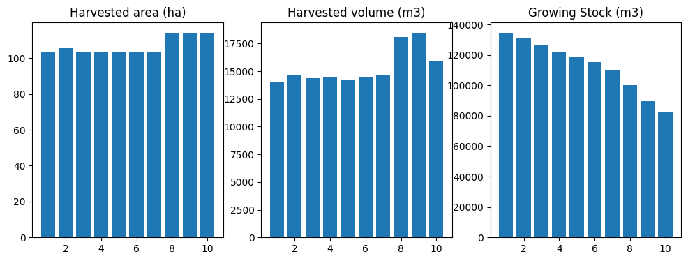
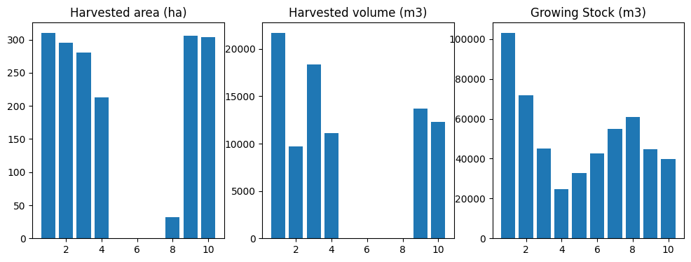
sch = schedule_harvest_areacontrol(fm)
[9]:
from util import compile_scenario, plot_scenario
df = compile_scenario(fm)
plot_scenario(df)
[9]:
(<Figure size 1200x400 with 3 Axes>,
 array([<Axes: title={'center': 'Harvested area (ha)'}>,
        <Axes: title={'center': 'Harvested volume (m3)'}>,
        <Axes: title={'center': 'Growing Stock (m3)'}>], dtype=object))

[10]:
disturbance_type_mapping = [{"user_dist_type": "harvest", "default_dist_type": "Clearcut harvesting without salvage"},
                            {"user_dist_type": "fire", "default_dist_type": "Wildfire"}]
[11]:
for dtype_key in fm.dtypes:
    fm.dt(dtype_key).last_pass_disturbance = "fire" if dtype_key[2] == dtype_key[4] else "harvest"
[12]:
sit_config, sit_tables = fm.to_cbm_sit(softwood_volume_yname="swdvol",
                                       hardwood_volume_yname="hwdvol",
                                       admin_boundary="British Columbia",
                                       eco_boundary="Montane Cordillera",
                                       disturbance_type_mapping=disturbance_type_mapping)
[13]:
fm.dt(("tsa24_clipped", "1", "2401002", "204", "2401002")).leading_species
[13]:
'softwood'
[14]:
fm = ws3.forest.ForestModel(model_name="tsa24_clipped",
                            model_path="data/woodstock_model_files_tsa24_clipped",
                            base_year=base_year,
                            horizon=horizon,
                            period_length=period_length,
                            max_age=max_age)
fm.import_landscape_section()
fm.import_areas_section(convert_periods_to_years=period_length)
fm.import_yields_section(convert_periods_to_years=period_length)
fm.import_actions_section(convert_periods_to_years=period_length)
fm.import_transitions_section(convert_periods_to_years=period_length)
fm.initialize_areas()
fm.add_null_action()
fm.reset_actions()
4.11.2. Export ws3 data to Standard Input Table (SIT) format
Export standard SIT tables from ws3 as a starting point.
[15]:
disturbance_type_mapping = [{"user_dist_type": "harvest", "default_dist_type": "Clearcut harvesting without salvage"},
                            {"user_dist_type": "fire", "default_dist_type": "Wildfire"}]
[16]:
for dtype_key in fm.dtypes:
    fm.dt(dtype_key).last_pass_disturbance = "fire" if dtype_key[2] == dtype_key[4] else "harvest"
[17]:
sit_config, sit_tables = fm.to_cbm_sit(softwood_volume_yname="swdvol",
                                       hardwood_volume_yname="hwdvol",
                                       admin_boundary="British Columbia",
                                       eco_boundary="Montane Cordillera",
                                       disturbance_type_mapping=disturbance_type_mapping)
[18]:
print(fm.dt(("tsa24_clipped", "1", "2402000", "100", "2422000")))
<ws3.forest.DevelopmentType object at 0x7d6e5efc60f0>
[19]:
p = fm.problems["__cbm_sit_bogus"]
for k in p.trees.keys(): print(k)
(('tsa24_clipped', '0', '2401000', '100', '2401000'), 85)
(('tsa24_clipped', '0', '2401000', '100', '2401000'), 95)
(('tsa24_clipped', '0', '2401000', '100', '2401000'), 105)
(('tsa24_clipped', '0', '2401000', '100', '2401000'), 125)
(('tsa24_clipped', '0', '2401000', '100', '2401000'), 135)
(('tsa24_clipped', '0', '2401000', '100', '2401000'), 145)
(('tsa24_clipped', '0', '2401000', '100', '2401000'), 155)
(('tsa24_clipped', '0', '2402005', '1201', '2402005'), 85)
(('tsa24_clipped', '1', '2401002', '204', '2401002'), 78)
(('tsa24_clipped', '1', '2401002', '204', '2401002'), 80)
(('tsa24_clipped', '1', '2401002', '204', '2401002'), 85)
(('tsa24_clipped', '1', '2401002', '204', '2401002'), 91)
(('tsa24_clipped', '1', '2401002', '204', '2401002'), 93)
(('tsa24_clipped', '1', '2401002', '204', '2401002'), 95)
(('tsa24_clipped', '1', '2401002', '204', '2401002'), 105)
(('tsa24_clipped', '1', '2401002', '204', '2401002'), 113)
(('tsa24_clipped', '1', '2401002', '204', '2401002'), 115)
(('tsa24_clipped', '1', '2401002', '204', '2401002'), 125)
(('tsa24_clipped', '1', '2401002', '204', '2401002'), 135)
(('tsa24_clipped', '1', '2401002', '204', '2401002'), 145)
(('tsa24_clipped', '1', '2401002', '204', '2401002'), 153)
(('tsa24_clipped', '1', '2401002', '204', '2401002'), 155)
(('tsa24_clipped', '1', '2401002', '204', '2421002'), 20)
(('tsa24_clipped', '1', '2402000', '100', '2402000'), 165)
(('tsa24_clipped', '1', '2402002', '204', '2402002'), 78)
(('tsa24_clipped', '1', '2402002', '204', '2402002'), 93)
(('tsa24_clipped', '1', '2402002', '204', '2402002'), 95)
(('tsa24_clipped', '1', '2402002', '204', '2402002'), 115)
(('tsa24_clipped', '1', '2403000', '100', '2403000'), 93)
(('tsa24_clipped', '1', '2403002', '204', '2403002'), 73)
(('tsa24_clipped', '1', '2403002', '204', '2423002'), 9)
(('tsa24_clipped', '1', '2403002', '204', '2423002'), 18)
[20]:
t = p.trees[(("tsa24_clipped", "1", "2402000", "100", "2402000"), 165)]
for path in t.paths():
    for n in path:
        print(n.data("dtk"))
    print()
('tsa24_clipped', '1', '2402000', '100', '2402000')
('tsa24_clipped', '1', '2402000', '100', '2422000')
('tsa24_clipped', '1', '2402000', '100', '2422000')
('tsa24_clipped', '1', '2402000', '100', '2422000')
('tsa24_clipped', '1', '2402000', '100', '2422000')
('tsa24_clipped', '1', '2402000', '100', '2422000')
('tsa24_clipped', '1', '2402000', '100', '2422000')
('tsa24_clipped', '1', '2402000', '100', '2422000')
('tsa24_clipped', '1', '2402000', '100', '2422000')
('tsa24_clipped', '1', '2402000', '100', '2422000')

('tsa24_clipped', '1', '2402000', '100', '2402000')
('tsa24_clipped', '1', '2402000', '100', '2402000')
('tsa24_clipped', '1', '2402000', '100', '2422000')
('tsa24_clipped', '1', '2402000', '100', '2422000')
('tsa24_clipped', '1', '2402000', '100', '2422000')
('tsa24_clipped', '1', '2402000', '100', '2422000')
('tsa24_clipped', '1', '2402000', '100', '2422000')
('tsa24_clipped', '1', '2402000', '100', '2422000')
('tsa24_clipped', '1', '2402000', '100', '2422000')
('tsa24_clipped', '1', '2402000', '100', '2422000')

('tsa24_clipped', '1', '2402000', '100', '2402000')
('tsa24_clipped', '1', '2402000', '100', '2402000')
('tsa24_clipped', '1', '2402000', '100', '2422000')
('tsa24_clipped', '1', '2402000', '100', '2422000')
('tsa24_clipped', '1', '2402000', '100', '2422000')
('tsa24_clipped', '1', '2402000', '100', '2422000')
('tsa24_clipped', '1', '2402000', '100', '2422000')
('tsa24_clipped', '1', '2402000', '100', '2422000')
('tsa24_clipped', '1', '2402000', '100', '2422000')
('tsa24_clipped', '1', '2402000', '100', '2422000')

('tsa24_clipped', '1', '2402000', '100', '2402000')
('tsa24_clipped', '1', '2402000', '100', '2402000')
('tsa24_clipped', '1', '2402000', '100', '2402000')
('tsa24_clipped', '1', '2402000', '100', '2422000')
('tsa24_clipped', '1', '2402000', '100', '2422000')
('tsa24_clipped', '1', '2402000', '100', '2422000')
('tsa24_clipped', '1', '2402000', '100', '2422000')
('tsa24_clipped', '1', '2402000', '100', '2422000')
('tsa24_clipped', '1', '2402000', '100', '2422000')
('tsa24_clipped', '1', '2402000', '100', '2422000')

('tsa24_clipped', '1', '2402000', '100', '2402000')
('tsa24_clipped', '1', '2402000', '100', '2402000')
('tsa24_clipped', '1', '2402000', '100', '2402000')
('tsa24_clipped', '1', '2402000', '100', '2402000')
('tsa24_clipped', '1', '2402000', '100', '2422000')
('tsa24_clipped', '1', '2402000', '100', '2422000')
('tsa24_clipped', '1', '2402000', '100', '2422000')
('tsa24_clipped', '1', '2402000', '100', '2422000')
('tsa24_clipped', '1', '2402000', '100', '2422000')
('tsa24_clipped', '1', '2402000', '100', '2422000')

('tsa24_clipped', '1', '2402000', '100', '2402000')
('tsa24_clipped', '1', '2402000', '100', '2402000')
('tsa24_clipped', '1', '2402000', '100', '2402000')
('tsa24_clipped', '1', '2402000', '100', '2402000')
('tsa24_clipped', '1', '2402000', '100', '2402000')
('tsa24_clipped', '1', '2402000', '100', '2422000')
('tsa24_clipped', '1', '2402000', '100', '2422000')
('tsa24_clipped', '1', '2402000', '100', '2422000')
('tsa24_clipped', '1', '2402000', '100', '2422000')
('tsa24_clipped', '1', '2402000', '100', '2422000')

('tsa24_clipped', '1', '2402000', '100', '2402000')
('tsa24_clipped', '1', '2402000', '100', '2402000')
('tsa24_clipped', '1', '2402000', '100', '2402000')
('tsa24_clipped', '1', '2402000', '100', '2402000')
('tsa24_clipped', '1', '2402000', '100', '2402000')
('tsa24_clipped', '1', '2402000', '100', '2402000')
('tsa24_clipped', '1', '2402000', '100', '2422000')
('tsa24_clipped', '1', '2402000', '100', '2422000')
('tsa24_clipped', '1', '2402000', '100', '2422000')
('tsa24_clipped', '1', '2402000', '100', '2422000')

('tsa24_clipped', '1', '2402000', '100', '2402000')
('tsa24_clipped', '1', '2402000', '100', '2402000')
('tsa24_clipped', '1', '2402000', '100', '2402000')
('tsa24_clipped', '1', '2402000', '100', '2402000')
('tsa24_clipped', '1', '2402000', '100', '2402000')
('tsa24_clipped', '1', '2402000', '100', '2402000')
('tsa24_clipped', '1', '2402000', '100', '2402000')
('tsa24_clipped', '1', '2402000', '100', '2422000')
('tsa24_clipped', '1', '2402000', '100', '2422000')
('tsa24_clipped', '1', '2402000', '100', '2422000')

('tsa24_clipped', '1', '2402000', '100', '2402000')
('tsa24_clipped', '1', '2402000', '100', '2402000')
('tsa24_clipped', '1', '2402000', '100', '2402000')
('tsa24_clipped', '1', '2402000', '100', '2402000')
('tsa24_clipped', '1', '2402000', '100', '2402000')
('tsa24_clipped', '1', '2402000', '100', '2402000')
('tsa24_clipped', '1', '2402000', '100', '2402000')
('tsa24_clipped', '1', '2402000', '100', '2402000')
('tsa24_clipped', '1', '2402000', '100', '2422000')
('tsa24_clipped', '1', '2402000', '100', '2422000')

('tsa24_clipped', '1', '2402000', '100', '2402000')
('tsa24_clipped', '1', '2402000', '100', '2402000')
('tsa24_clipped', '1', '2402000', '100', '2402000')
('tsa24_clipped', '1', '2402000', '100', '2402000')
('tsa24_clipped', '1', '2402000', '100', '2402000')
('tsa24_clipped', '1', '2402000', '100', '2402000')
('tsa24_clipped', '1', '2402000', '100', '2402000')
('tsa24_clipped', '1', '2402000', '100', '2402000')
('tsa24_clipped', '1', '2402000', '100', '2402000')
('tsa24_clipped', '1', '2402000', '100', '2402000')

('tsa24_clipped', '1', '2402000', '100', '2402000')
('tsa24_clipped', '1', '2402000', '100', '2402000')
('tsa24_clipped', '1', '2402000', '100', '2402000')
('tsa24_clipped', '1', '2402000', '100', '2402000')
('tsa24_clipped', '1', '2402000', '100', '2402000')
('tsa24_clipped', '1', '2402000', '100', '2402000')
('tsa24_clipped', '1', '2402000', '100', '2402000')
('tsa24_clipped', '1', '2402000', '100', '2402000')
('tsa24_clipped', '1', '2402000', '100', '2402000')
('tsa24_clipped', '1', '2402000', '100', '2402000')
The sit_events table should be empty, because we did not simulate any actions before calling fm.to_cbm_sit.
[21]:
sit_tables["sit_events"]
[21]:
| theme0 | theme1 | theme2 | theme3 | theme4 | species | using_age_class | min_softwood_age | max_softwood_age | min_hardwood_age | ... | MinSWMerchStemSnagC | MaxSWMerchStemSnagC | MinHWMerchStemSnagC | MaxHWMerchStemSnagC | efficiency | sort_type | target_type | target | disturbance_type | disturbance_year |
|---|
0 rows × 38 columns
Rebuild the inventory table. We need one inventory record for every possible development type (including system states that are not present in the initial inventory). Conveniently for us, fm.to_cbm_sit calls fm._cbm_sit_yield, which calls fm.add_problem, which calls fm._bld_tree_m1, which simulates all feasible combinations of actions, which creates any new development types that we need. You just have to know, and now you can leverage that side-effect to make this next part
easy peasy.
Figuring out which development types were missing and adding them by hand would not have been too difficult for the simple test dataset we are are using here (assuming you are good at reading Woodstock input files and running through all possible future states in your head), but this could be a doozie of a puzzle or larger models with hundreds of initial development types and more complex actions and transitions. Basically, you definitely want to take note of the add_problem hack described
about and use that. Any other way is just looking for trouble.
We can reuse the sit_inventory table returned from fm.to_cbm_sit to make sure we have the correct structure.
[22]:
df = sit_tables["sit_inventory"]
df = df.iloc[0:0]
df
[22]:
| theme0 | theme1 | theme2 | theme3 | theme4 | species | using_age_class | age | area | delay | landclass | historic_disturbance | last_pass_disturbance |
|---|
[23]:
import pandas as pd
[24]:
data = []
for dtype_key in fm.dtypes:
    dt = fm.dt(dtype_key)
    values = list(dtype_key)
    values += [dt.leading_species, "FALSE", 0, 1., 0, 0, "fire", "fire" if dtype_key[2] == dtype_key[4] else "harvest"]
    data.append(dict(zip(df.columns, values)))
sit_tables["sit_inventory"] = pd.DataFrame(data)
sit_tables["sit_inventory"]
[24]:
| theme0 | theme1 | theme2 | theme3 | theme4 | species | using_age_class | age | area | delay | landclass | historic_disturbance | last_pass_disturbance | |
|---|---|---|---|---|---|---|---|---|---|---|---|---|---|
| 0 | tsa24_clipped | 0 | 2401000 | 100 | 2401000 | softwood | FALSE | 0 | 1.0 | 0 | 0 | fire | fire |
| 1 | tsa24_clipped | 0 | 2402005 | 1201 | 2402005 | hardwood | FALSE | 0 | 1.0 | 0 | 0 | fire | fire |
| 2 | tsa24_clipped | 1 | 2401002 | 204 | 2401002 | softwood | FALSE | 0 | 1.0 | 0 | 0 | fire | fire |
| 3 | tsa24_clipped | 1 | 2401002 | 204 | 2421002 | softwood | FALSE | 0 | 1.0 | 0 | 0 | fire | harvest |
| 4 | tsa24_clipped | 1 | 2402000 | 100 | 2402000 | softwood | FALSE | 0 | 1.0 | 0 | 0 | fire | fire |
| 5 | tsa24_clipped | 1 | 2402002 | 204 | 2402002 | softwood | FALSE | 0 | 1.0 | 0 | 0 | fire | fire |
| 6 | tsa24_clipped | 1 | 2403000 | 100 | 2403000 | softwood | FALSE | 0 | 1.0 | 0 | 0 | fire | fire |
| 7 | tsa24_clipped | 1 | 2403002 | 204 | 2403002 | softwood | FALSE | 0 | 1.0 | 0 | 0 | fire | fire |
| 8 | tsa24_clipped | 1 | 2403002 | 204 | 2423002 | softwood | FALSE | 0 | 1.0 | 0 | 0 | fire | harvest |
| 9 | tsa24_clipped | 1 | 2402000 | 100 | 2422000 | softwood | FALSE | 0 | 1.0 | 0 | 0 | fire | harvest |
| 10 | tsa24_clipped | 1 | 2402002 | 204 | 2422002 | softwood | FALSE | 0 | 1.0 | 0 | 0 | fire | harvest |
| 11 | tsa24_clipped | 1 | 2403000 | 100 | 2423000 | softwood | FALSE | 0 | 1.0 | 0 | 0 | fire | harvest |
4.11.3. Run CBM using built-in ws3 functions
Now we run this thruogh libcbm for 300 time steps.
[25]:
disturbance_type_mapping = [{"user_dist_type": "harvest", "default_dist_type": "Clearcut harvesting without salvage"},
                            {"user_dist_type": "fire", "default_dist_type": "Wildfire"}]
[26]:
for dtype_key in fm.dtypes:
    fm.dt(dtype_key).last_pass_disturbance = "fire" if dtype_key[2] == dtype_key[4] else "harvest"
[27]:
from util import run_cbm
[28]:
n_steps = 300
cbm_output = run_cbm(sit_config, sit_tables, n_steps, plot=False)
[29]:
cbm_output
[29]:
<libcbm.model.cbm.cbm_output.CBMOutput at 0x7d6e5f17a2a0>
[30]:
pi = cbm_output.classifiers.to_pandas().merge(cbm_output.pools.to_pandas(),
                                              left_on=["identifier", "timestep"],
                                              right_on=["identifier", "timestep"])
fi = cbm_output.classifiers.to_pandas().merge(cbm_output.flux.to_pandas(),
                                              left_on=["identifier", "timestep"],
                                              right_on=["identifier", "timestep"])
[31]:
pi
[31]:
| identifier | timestep | theme0 | theme1 | theme2 | theme3 | theme4 | species | Input | SoftwoodMerch | ... | BelowGroundSlowSoil | SoftwoodStemSnag | SoftwoodBranchSnag | HardwoodStemSnag | HardwoodBranchSnag | CO2 | CH4 | CO | NO2 | Products | |
|---|---|---|---|---|---|---|---|---|---|---|---|---|---|---|---|---|---|---|---|---|---|
| 0 | 1 | 0 | tsa24_clipped | 0 | 2401000 | 100 | 2401000 | softwood | 1.0 | 0.000000 | ... | 61.072161 | 28.616202 | 19.461734 | 0.000000 | 0.000000 | 4790.526504 | 4.942348 | 44.479699 | 0.0 | 0.000000 |
| 1 | 2 | 0 | tsa24_clipped | 0 | 2402005 | 1201 | 2402005 | hardwood | 1.0 | 0.000000 | ... | 114.491754 | 0.000000 | 0.000000 | 65.448939 | 18.985542 | 9638.462743 | 8.550696 | 76.954017 | 0.0 | 0.000000 |
| 2 | 3 | 0 | tsa24_clipped | 1 | 2401002 | 204 | 2401002 | softwood | 1.0 | 0.000000 | ... | 70.577311 | 38.209170 | 20.940326 | 0.000000 | 0.000000 | 5549.131806 | 5.574412 | 50.168153 | 0.0 | 0.000000 |
| 3 | 4 | 0 | tsa24_clipped | 1 | 2401002 | 204 | 2421002 | softwood | 1.0 | 0.000000 | ... | 56.591833 | 0.000000 | 0.000000 | 0.000000 | 0.000000 | 4504.469208 | 4.878363 | 43.903950 | 0.0 | 34.110922 |
| 4 | 5 | 0 | tsa24_clipped | 1 | 2402000 | 100 | 2402000 | softwood | 1.0 | 0.000000 | ... | 78.415619 | 47.913734 | 22.404296 | 0.000000 | 0.000000 | 6182.050833 | 6.060943 | 54.546827 | 0.0 | 0.000000 |
| ... | ... | ... | ... | ... | ... | ... | ... | ... | ... | ... | ... | ... | ... | ... | ... | ... | ... | ... | ... | ... | ... |
| 3607 | 8 | 300 | tsa24_clipped | 1 | 2403002 | 204 | 2403002 | softwood | 1.0 | 63.042997 | ... | 110.566427 | 10.465389 | 1.954894 | 0.000000 | 0.000000 | 9088.654777 | 7.694727 | 69.250637 | 0.0 | 0.000000 |
| 3608 | 9 | 300 | tsa24_clipped | 1 | 2403002 | 204 | 2423002 | softwood | 1.0 | 92.723531 | ... | 118.471450 | 9.851096 | 2.270104 | 0.000000 | 0.000000 | 9070.482693 | 7.597707 | 68.377586 | 0.0 | 79.633546 |
| 3609 | 10 | 300 | tsa24_clipped | 1 | 2402000 | 100 | 2422000 | softwood | 1.0 | 74.795270 | ... | 87.528498 | 7.785973 | 2.065819 | 0.000000 | 0.000000 | 6201.980905 | 5.599995 | 50.398516 | 0.0 | 48.597173 |
| 3610 | 11 | 300 | tsa24_clipped | 1 | 2402002 | 204 | 2422002 | softwood | 1.0 | 66.253514 | ... | 93.752506 | 6.990460 | 1.970435 | 0.000000 | 0.000000 | 6923.626178 | 6.063782 | 54.572506 | 0.0 | 53.757580 |
| 3611 | 12 | 300 | tsa24_clipped | 1 | 2403000 | 100 | 2423000 | softwood | 1.0 | 93.686522 | ... | 106.682383 | 9.854980 | 2.280876 | 0.000000 | 0.000000 | 7881.389804 | 6.779255 | 61.011651 | 0.0 | 68.419040 |
3612 rows × 35 columns
[32]:
pi.columns
[32]:
Index(['identifier', 'timestep', 'theme0', 'theme1', 'theme2', 'theme3',
       'theme4', 'species', 'Input', 'SoftwoodMerch', 'SoftwoodFoliage',
       'SoftwoodOther', 'SoftwoodCoarseRoots', 'SoftwoodFineRoots',
       'HardwoodMerch', 'HardwoodFoliage', 'HardwoodOther',
       'HardwoodCoarseRoots', 'HardwoodFineRoots', 'AboveGroundVeryFastSoil',
       'BelowGroundVeryFastSoil', 'AboveGroundFastSoil', 'BelowGroundFastSoil',
       'MediumSoil', 'AboveGroundSlowSoil', 'BelowGroundSlowSoil',
       'SoftwoodStemSnag', 'SoftwoodBranchSnag', 'HardwoodStemSnag',
       'HardwoodBranchSnag', 'CO2', 'CH4', 'CO', 'NO2', 'Products'],
      dtype='object')
[33]:
fi
[33]:
| identifier | timestep | theme0 | theme1 | theme2 | theme3 | theme4 | species | DisturbanceCO2Production | DisturbanceCH4Production | ... | DisturbanceVFastBGToAir | DisturbanceFastAGToAir | DisturbanceFastBGToAir | DisturbanceMediumToAir | DisturbanceSlowAGToAir | DisturbanceSlowBGToAir | DisturbanceSWStemSnagToAir | DisturbanceSWBranchSnagToAir | DisturbanceHWStemSnagToAir | DisturbanceHWBranchSnagToAir | |
|---|---|---|---|---|---|---|---|---|---|---|---|---|---|---|---|---|---|---|---|---|---|
| 0 | 1 | 0 | tsa24_clipped | 0 | 2401000 | 100 | 2401000 | softwood | 0.0 | 0.0 | ... | 0.0 | 0.0 | 0.0 | 0.0 | 0.0 | 0.0 | 0.0 | 0.0 | 0.0 | 0.0 |
| 1 | 2 | 0 | tsa24_clipped | 0 | 2402005 | 1201 | 2402005 | hardwood | 0.0 | 0.0 | ... | 0.0 | 0.0 | 0.0 | 0.0 | 0.0 | 0.0 | 0.0 | 0.0 | 0.0 | 0.0 |
| 2 | 3 | 0 | tsa24_clipped | 1 | 2401002 | 204 | 2401002 | softwood | 0.0 | 0.0 | ... | 0.0 | 0.0 | 0.0 | 0.0 | 0.0 | 0.0 | 0.0 | 0.0 | 0.0 | 0.0 |
| 3 | 4 | 0 | tsa24_clipped | 1 | 2401002 | 204 | 2421002 | softwood | 0.0 | 0.0 | ... | 0.0 | 0.0 | 0.0 | 0.0 | 0.0 | 0.0 | 0.0 | 0.0 | 0.0 | 0.0 |
| 4 | 5 | 0 | tsa24_clipped | 1 | 2402000 | 100 | 2402000 | softwood | 0.0 | 0.0 | ... | 0.0 | 0.0 | 0.0 | 0.0 | 0.0 | 0.0 | 0.0 | 0.0 | 0.0 | 0.0 |
| ... | ... | ... | ... | ... | ... | ... | ... | ... | ... | ... | ... | ... | ... | ... | ... | ... | ... | ... | ... | ... | ... |
| 3607 | 8 | 300 | tsa24_clipped | 1 | 2403002 | 204 | 2403002 | softwood | 0.0 | 0.0 | ... | 0.0 | 0.0 | 0.0 | 0.0 | 0.0 | 0.0 | 0.0 | 0.0 | 0.0 | 0.0 |
| 3608 | 9 | 300 | tsa24_clipped | 1 | 2403002 | 204 | 2423002 | softwood | 0.0 | 0.0 | ... | 0.0 | 0.0 | 0.0 | 0.0 | 0.0 | 0.0 | 0.0 | 0.0 | 0.0 | 0.0 |
| 3609 | 10 | 300 | tsa24_clipped | 1 | 2402000 | 100 | 2422000 | softwood | 0.0 | 0.0 | ... | 0.0 | 0.0 | 0.0 | 0.0 | 0.0 | 0.0 | 0.0 | 0.0 | 0.0 | 0.0 |
| 3610 | 11 | 300 | tsa24_clipped | 1 | 2402002 | 204 | 2422002 | softwood | 0.0 | 0.0 | ... | 0.0 | 0.0 | 0.0 | 0.0 | 0.0 | 0.0 | 0.0 | 0.0 | 0.0 | 0.0 |
| 3611 | 12 | 300 | tsa24_clipped | 1 | 2403000 | 100 | 2423000 | softwood | 0.0 | 0.0 | ... | 0.0 | 0.0 | 0.0 | 0.0 | 0.0 | 0.0 | 0.0 | 0.0 | 0.0 | 0.0 |
3612 rows × 60 columns
[34]:
fi.columns
[34]:
Index(['identifier', 'timestep', 'theme0', 'theme1', 'theme2', 'theme3',
       'theme4', 'species', 'DisturbanceCO2Production',
       'DisturbanceCH4Production', 'DisturbanceCOProduction',
       'DisturbanceBioCO2Emission', 'DisturbanceBioCH4Emission',
       'DisturbanceBioCOEmission', 'DecayDOMCO2Emission',
       'DisturbanceSoftProduction', 'DisturbanceHardProduction',
       'DisturbanceDOMProduction', 'DeltaBiomass_AG', 'DeltaBiomass_BG',
       'TurnoverMerchLitterInput', 'TurnoverFolLitterInput',
       'TurnoverOthLitterInput', 'TurnoverCoarseLitterInput',
       'TurnoverFineLitterInput', 'DecayVFastAGToAir', 'DecayVFastBGToAir',
       'DecayFastAGToAir', 'DecayFastBGToAir', 'DecayMediumToAir',
       'DecaySlowAGToAir', 'DecaySlowBGToAir', 'DecaySWStemSnagToAir',
       'DecaySWBranchSnagToAir', 'DecayHWStemSnagToAir',
       'DecayHWBranchSnagToAir', 'DisturbanceMerchToAir',
       'DisturbanceFolToAir', 'DisturbanceOthToAir', 'DisturbanceCoarseToAir',
       'DisturbanceFineToAir', 'DisturbanceDOMCO2Emission',
       'DisturbanceDOMCH4Emission', 'DisturbanceDOMCOEmission',
       'DisturbanceMerchLitterInput', 'DisturbanceFolLitterInput',
       'DisturbanceOthLitterInput', 'DisturbanceCoarseLitterInput',
       'DisturbanceFineLitterInput', 'DisturbanceVFastAGToAir',
       'DisturbanceVFastBGToAir', 'DisturbanceFastAGToAir',
       'DisturbanceFastBGToAir', 'DisturbanceMediumToAir',
       'DisturbanceSlowAGToAir', 'DisturbanceSlowBGToAir',
       'DisturbanceSWStemSnagToAir', 'DisturbanceSWBranchSnagToAir',
       'DisturbanceHWStemSnagToAir', 'DisturbanceHWBranchSnagToAir'],
      dtype='object')
4.11.4. Import CBM output back into ws3 (as carbon yield curves)
Now we just need to recompile this data into yield curves and stuff them back into our ForestModel instance.
[35]:
biomass_pools = ["SoftwoodMerch","SoftwoodFoliage", "SoftwoodOther", "SoftwoodCoarseRoots","SoftwoodFineRoots",
                 "HardwoodMerch", "HardwoodFoliage", "HardwoodOther", "HardwoodCoarseRoots", "HardwoodFineRoots"]
dom_pools = ["AboveGroundVeryFastSoil", "BelowGroundVeryFastSoil", "AboveGroundFastSoil", "BelowGroundFastSoil",
             "MediumSoil", "AboveGroundSlowSoil", "BelowGroundSlowSoil", "SoftwoodStemSnag", "SoftwoodBranchSnag",
             "HardwoodStemSnag", "HardwoodBranchSnag"]
emissions_pools = ["CO2", "CH4", "CO", "NO2"]
products_pools = ["Products"]
ecosystem_pools = biomass_pools + dom_pools
all_pools = biomass_pools + dom_pools + emissions_pools + products_pools
[36]:
annual_process_fluxes = [
    "DecayDOMCO2Emission",
    "DeltaBiomass_AG",
    "DeltaBiomass_BG",
    "TurnoverMerchLitterInput",
    "TurnoverFolLitterInput",
    "TurnoverOthLitterInput",
    "TurnoverCoarseLitterInput",
    "TurnoverFineLitterInput",
    "DecayVFastAGToAir",
    "DecayVFastBGToAir",
    "DecayFastAGToAir",
    "DecayFastBGToAir",
    "DecayMediumToAir",
    "DecaySlowAGToAir",
    "DecaySlowBGToAir",
    "DecaySWStemSnagToAir",
    "DecaySWBranchSnagToAir",
    "DecayHWStemSnagToAir",
    "DecayHWBranchSnagToAir"
]

npp_fluxes=[
    "DeltaBiomass_AG",
    "DeltaBiomass_BG"
]
decay_emissions_fluxes = [
    "DecayVFastAGToAir",
    "DecayVFastBGToAir",
    "DecayFastAGToAir",
    "DecayFastBGToAir",
    "DecayMediumToAir",
    "DecaySlowAGToAir",
    "DecaySlowBGToAir",
    "DecaySWStemSnagToAir",
    "DecaySWBranchSnagToAir",
    "DecayHWStemSnagToAir",
    "DecayHWBranchSnagToAir"
]

disturbance_production_fluxes = [
    "DisturbanceSoftProduction",
    "DisturbanceHardProduction",
    "DisturbanceDOMProduction"
]

disturbance_emissions_fluxes = [
    "DisturbanceMerchToAir",
    "DisturbanceFolToAir",
    "DisturbanceOthToAir",
    "DisturbanceCoarseToAir",
    "DisturbanceFineToAir",
    "DisturbanceVFastAGToAir",
    "DisturbanceVFastBGToAir",
    "DisturbanceFastAGToAir",
    "DisturbanceFastBGToAir",
    "DisturbanceMediumToAir",
    "DisturbanceSlowAGToAir",
    "DisturbanceSlowBGToAir",
    "DisturbanceSWStemSnagToAir",
    "DisturbanceSWBranchSnagToAir",
    "DisturbanceHWStemSnagToAir",
    "DisturbanceHWBranchSnagToAir"
]

all_fluxes = [
    "DisturbanceCO2Production",
    "DisturbanceCH4Production",
    "DisturbanceCOProduction",
    "DisturbanceBioCO2Emission",
    "DisturbanceBioCH4Emission",
    "DisturbanceBioCOEmission",
    "DecayDOMCO2Emission",
    "DisturbanceSoftProduction",
    "DisturbanceHardProduction",
    "DisturbanceDOMProduction",
    "DeltaBiomass_AG",
    "DeltaBiomass_BG",
    "TurnoverMerchLitterInput",
    "TurnoverFolLitterInput",
    "TurnoverOthLitterInput",
    "TurnoverCoarseLitterInput",
    "TurnoverFineLitterInput",
    "DecayVFastAGToAir",
    "DecayVFastBGToAir",
    "DecayFastAGToAir",
    "DecayFastBGToAir",
    "DecayMediumToAir",
    "DecaySlowAGToAir",
    "DecaySlowBGToAir",
    "DecaySWStemSnagToAir",
    "DecaySWBranchSnagToAir",
    "DecayHWStemSnagToAir",
    "DecayHWBranchSnagToAir",
    "DisturbanceMerchToAir",
    "DisturbanceFolToAir",
    "DisturbanceOthToAir",
    "DisturbanceCoarseToAir",
    "DisturbanceFineToAir",
    "DisturbanceDOMCO2Emission",
    "DisturbanceDOMCH4Emission",
    "DisturbanceDOMCOEmission",
    "DisturbanceMerchLitterInput",
    "DisturbanceFolLitterInput",
    "DisturbanceOthLitterInput",
    "DisturbanceCoarseLitterInput",
    "DisturbanceFineLitterInput",
    "DisturbanceVFastAGToAir",
    "DisturbanceVFastBGToAir",
    "DisturbanceFastAGToAir",
    "DisturbanceFastBGToAir",
    "DisturbanceMediumToAir",
    "DisturbanceSlowAGToAir",
    "DisturbanceSlowBGToAir",
    "DisturbanceSWStemSnagToAir",
    "DisturbanceSWBranchSnagToAir",
    "DisturbanceHWStemSnagToAir",
    "DisturbanceHWBranchSnagToAir"
]
[37]:
pi["dtype_key"] = pi.apply(lambda r: "%s %s %s %s %s" % (r["theme0"], r["theme1"], r["theme2"], r["theme3"], r["theme4"]), axis=1)
fi["dtype_key"] = fi.apply(lambda r: "%s %s %s %s %s" % (r["theme0"], r["theme1"], r["theme2"], r["theme3"], r["theme4"]), axis=1)
[38]:
pi_gb_sum = pi.groupby(["dtype_key", "timestep"], as_index=True)[all_pools].sum()
fi_gb_sum = fi.groupby(["dtype_key", "timestep"], as_index=True)[all_fluxes].sum()
Reformatted this way, we essentially have carbon yield curves now.
[39]:
pi_gb_sum
[39]:
| SoftwoodMerch | SoftwoodFoliage | SoftwoodOther | SoftwoodCoarseRoots | SoftwoodFineRoots | HardwoodMerch | HardwoodFoliage | HardwoodOther | HardwoodCoarseRoots | HardwoodFineRoots | ... | BelowGroundSlowSoil | SoftwoodStemSnag | SoftwoodBranchSnag | HardwoodStemSnag | HardwoodBranchSnag | CO2 | CH4 | CO | NO2 | Products | ||
|---|---|---|---|---|---|---|---|---|---|---|---|---|---|---|---|---|---|---|---|---|---|---|
| dtype_key | timestep | |||||||||||||||||||||
| tsa24_clipped 0 2401000 100 2401000 | 0 | 0.000000 | 0.000000 | 0.000000 | 0.000000 | 0.000000 | 0.0 | 0.0 | 0.0 | 0.0 | 0.0 | ... | 61.072161 | 28.616202 | 19.461734 | 0.0 | 0.0 | 4790.526504 | 4.942348 | 44.479699 | 0.0 | 0.000000 |
| 1 | 0.000036 | 0.132721 | 0.000000 | 0.016954 | 0.012518 | 0.0 | 0.0 | 0.0 | 0.0 | 0.0 | ... | 61.121090 | 27.409295 | 16.809097 | 0.0 | 0.0 | 4793.580328 | 4.942348 | 44.479699 | 0.0 | 0.000000 | |
| 2 | 0.000305 | 0.370208 | 0.000000 | 0.047501 | 0.034753 | 0.0 | 0.0 | 0.0 | 0.0 | 0.0 | ... | 61.131684 | 26.253292 | 14.518014 | 0.0 | 0.0 | 4796.408697 | 4.942348 | 44.479699 | 0.0 | 0.000000 | |
| 3 | 0.001061 | 0.611266 | 0.061592 | 0.086822 | 0.062788 | 0.0 | 0.0 | 0.0 | 0.0 | 0.0 | ... | 61.114167 | 25.146046 | 12.539502 | 0.0 | 0.0 | 4799.057094 | 4.942348 | 44.479699 | 0.0 | 0.000000 | |
| 4 | 0.002569 | 0.774699 | 0.251065 | 0.133230 | 0.095060 | 0.0 | 0.0 | 0.0 | 0.0 | 0.0 | ... | 61.076059 | 24.085504 | 10.831866 | 0.0 | 0.0 | 4801.559391 | 4.942348 | 44.479699 | 0.0 | 0.000000 | |
| ... | ... | ... | ... | ... | ... | ... | ... | ... | ... | ... | ... | ... | ... | ... | ... | ... | ... | ... | ... | ... | ... | ... |
| tsa24_clipped 1 2403002 204 2423002 | 296 | 92.723531 | 8.635211 | 32.241928 | 27.228756 | 2.430592 | 0.0 | 0.0 | 0.0 | 0.0 | 0.0 | ... | 118.137520 | 9.862722 | 2.270108 | 0.0 | 0.0 | 9052.158176 | 7.597707 | 68.377586 | 0.0 | 79.633546 |
| 297 | 92.723531 | 8.635211 | 32.241928 | 27.228756 | 2.430592 | 0.0 | 0.0 | 0.0 | 0.0 | 0.0 | ... | 118.221284 | 9.859625 | 2.270107 | 0.0 | 0.0 | 9056.738888 | 7.597707 | 68.377586 | 0.0 | 79.633546 | |
| 298 | 92.723531 | 8.635211 | 32.241928 | 27.228756 | 2.430592 | 0.0 | 0.0 | 0.0 | 0.0 | 0.0 | ... | 118.304861 | 9.856659 | 2.270106 | 0.0 | 0.0 | 9061.319879 | 7.597707 | 68.377586 | 0.0 | 79.633546 | |
| 299 | 92.723531 | 8.635211 | 32.241928 | 27.228756 | 2.430592 | 0.0 | 0.0 | 0.0 | 0.0 | 0.0 | ... | 118.388250 | 9.853818 | 2.270105 | 0.0 | 0.0 | 9065.901147 | 7.597707 | 68.377586 | 0.0 | 79.633546 | |
| 300 | 92.723531 | 8.635211 | 32.241928 | 27.228756 | 2.430592 | 0.0 | 0.0 | 0.0 | 0.0 | 0.0 | ... | 118.471450 | 9.851096 | 2.270104 | 0.0 | 0.0 | 9070.482693 | 7.597707 | 68.377586 | 0.0 | 79.633546 |
3612 rows × 26 columns
[40]:
fi_gb_sum
[40]:
| DisturbanceCO2Production | DisturbanceCH4Production | DisturbanceCOProduction | DisturbanceBioCO2Emission | DisturbanceBioCH4Emission | DisturbanceBioCOEmission | DecayDOMCO2Emission | DisturbanceSoftProduction | DisturbanceHardProduction | DisturbanceDOMProduction | ... | DisturbanceVFastBGToAir | DisturbanceFastAGToAir | DisturbanceFastBGToAir | DisturbanceMediumToAir | DisturbanceSlowAGToAir | DisturbanceSlowBGToAir | DisturbanceSWStemSnagToAir | DisturbanceSWBranchSnagToAir | DisturbanceHWStemSnagToAir | DisturbanceHWBranchSnagToAir | ||
|---|---|---|---|---|---|---|---|---|---|---|---|---|---|---|---|---|---|---|---|---|---|---|
| dtype_key | timestep | |||||||||||||||||||||
| tsa24_clipped 0 2401000 100 2401000 | 0 | 0.0 | 0.0 | 0.0 | 0.0 | 0.0 | 0.0 | 0.000000 | 0.0 | 0.0 | 0.0 | ... | 0.0 | 0.0 | 0.0 | 0.0 | 0.0 | 0.0 | 0.0 | 0.0 | 0.0 | 0.0 |
| 1 | 0.0 | 0.0 | 0.0 | 0.0 | 0.0 | 0.0 | 3.053824 | 0.0 | 0.0 | 0.0 | ... | 0.0 | 0.0 | 0.0 | 0.0 | 0.0 | 0.0 | 0.0 | 0.0 | 0.0 | 0.0 | |
| 2 | 0.0 | 0.0 | 0.0 | 0.0 | 0.0 | 0.0 | 2.828369 | 0.0 | 0.0 | 0.0 | ... | 0.0 | 0.0 | 0.0 | 0.0 | 0.0 | 0.0 | 0.0 | 0.0 | 0.0 | 0.0 | |
| 3 | 0.0 | 0.0 | 0.0 | 0.0 | 0.0 | 0.0 | 2.648398 | 0.0 | 0.0 | 0.0 | ... | 0.0 | 0.0 | 0.0 | 0.0 | 0.0 | 0.0 | 0.0 | 0.0 | 0.0 | 0.0 | |
| 4 | 0.0 | 0.0 | 0.0 | 0.0 | 0.0 | 0.0 | 2.502297 | 0.0 | 0.0 | 0.0 | ... | 0.0 | 0.0 | 0.0 | 0.0 | 0.0 | 0.0 | 0.0 | 0.0 | 0.0 | 0.0 | |
| ... | ... | ... | ... | ... | ... | ... | ... | ... | ... | ... | ... | ... | ... | ... | ... | ... | ... | ... | ... | ... | ... | ... |
| tsa24_clipped 1 2403002 204 2423002 | 296 | 0.0 | 0.0 | 0.0 | 0.0 | 0.0 | 0.0 | 4.580435 | 0.0 | 0.0 | 0.0 | ... | 0.0 | 0.0 | 0.0 | 0.0 | 0.0 | 0.0 | 0.0 | 0.0 | 0.0 | 0.0 |
| 297 | 0.0 | 0.0 | 0.0 | 0.0 | 0.0 | 0.0 | 4.580713 | 0.0 | 0.0 | 0.0 | ... | 0.0 | 0.0 | 0.0 | 0.0 | 0.0 | 0.0 | 0.0 | 0.0 | 0.0 | 0.0 | |
| 298 | 0.0 | 0.0 | 0.0 | 0.0 | 0.0 | 0.0 | 4.580990 | 0.0 | 0.0 | 0.0 | ... | 0.0 | 0.0 | 0.0 | 0.0 | 0.0 | 0.0 | 0.0 | 0.0 | 0.0 | 0.0 | |
| 299 | 0.0 | 0.0 | 0.0 | 0.0 | 0.0 | 0.0 | 4.581268 | 0.0 | 0.0 | 0.0 | ... | 0.0 | 0.0 | 0.0 | 0.0 | 0.0 | 0.0 | 0.0 | 0.0 | 0.0 | 0.0 | |
| 300 | 0.0 | 0.0 | 0.0 | 0.0 | 0.0 | 0.0 | 4.581546 | 0.0 | 0.0 | 0.0 | ... | 0.0 | 0.0 | 0.0 | 0.0 | 0.0 | 0.0 | 0.0 | 0.0 | 0.0 | 0.0 |
3612 rows × 52 columns
Add carbon yield curves to our model.
[41]:
for dtype_key in fm.dtypes:
    dt = fm.dt(dtype_key)
    mask = ("?", "?", dtype_key[2], "?", dtype_key[4])
    for _mask, ytype, curves in fm.yields:
        if _mask != mask: continue # we know there will be a match so this works
        print("found match for mask", mask)
        pool_data = pi_gb_sum.loc[" ".join(dtype_key)]
        for yname in all_pools:
            points = list(zip(pool_data.index.values, pool_data[yname]))
            curve = fm.register_curve(ws3.core.Curve(yname,
                                                     points=points,
                                                     type="a",
                                                     is_volume=False,
                                                     xmax=fm.max_age,
                                                     period_length=fm.period_length))
            curves.append((yname, curve))
            dt.add_ycomp("a", yname, curve)
        flux_data = fi_gb_sum.loc[" ".join(dtype_key)]
        for yname in all_fluxes:
            points = list(zip(flux_data.index.values, flux_data[yname]))
            curve = fm.register_curve(ws3.core.Curve(yname,
                                                     points=points,
                                                     type="a",
                                                     is_volume=False,
                                                     xmax=fm.max_age,
                                                     period_length=fm.period_length))
            curves.append((yname, curve))
            dt.add_ycomp("a", yname, curve)
found match for mask ('?', '?', '2401000', '?', '2401000')
found match for mask ('?', '?', '2401000', '?', '2401000')
found match for mask ('?', '?', '2402005', '?', '2402005')
found match for mask ('?', '?', '2402005', '?', '2402005')
found match for mask ('?', '?', '2401002', '?', '2401002')
found match for mask ('?', '?', '2401002', '?', '2421002')
found match for mask ('?', '?', '2402000', '?', '2402000')
found match for mask ('?', '?', '2402002', '?', '2402002')
found match for mask ('?', '?', '2403000', '?', '2403000')
found match for mask ('?', '?', '2403002', '?', '2403002')
found match for mask ('?', '?', '2403002', '?', '2423002')
found match for mask ('?', '?', '2402000', '?', '2422000')
found match for mask ('?', '?', '2402002', '?', '2422002')
found match for mask ('?', '?', '2403000', '?', '2423000')
[42]:
fm.reset()
[43]:
fm.grow()
[44]:
import matplotlib.pyplot as plt
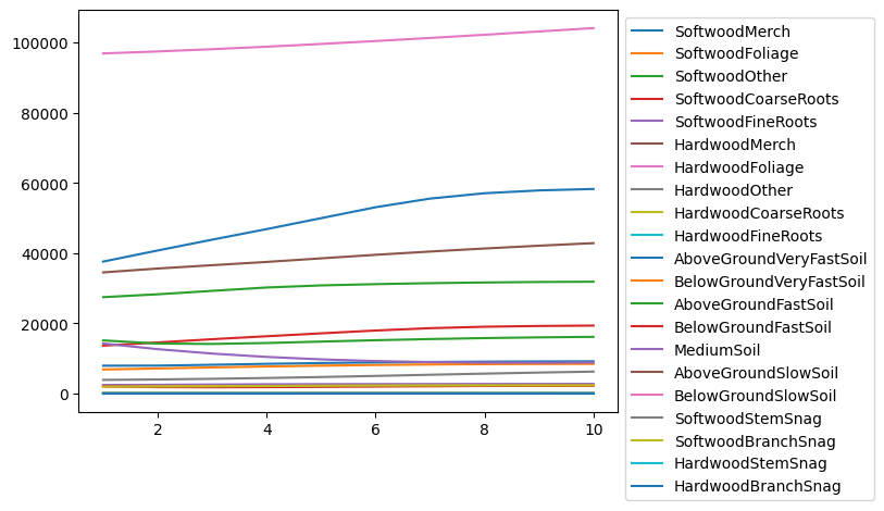
for pool in ecosystem_pools:
x, y = fm.periods, [fm.inventory(p, pool) for p in fm.periods]
plt.plot(x, y, label=pool)
plt.legend(bbox_to_anchor=(1, 1))
[44]:
<matplotlib.legend.Legend at 0x7d6e5f09dbe0>
[45]:
import matplotlib.pyplot as plt
for flux in annual_process_fluxes:
    x, y = fm.periods, [fm.inventory(p, flux) for p in fm.periods]
    plt.plot(x, y, label=flux)
plt.legend(bbox_to_anchor=(1, 1))
[45]:
<matplotlib.legend.Legend at 0x7d6e6136f4a0>
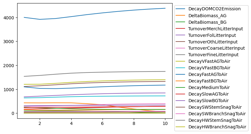
Not the most pretty or informative plots, but the point is that we are new tracking 26 new carbon pools and 52 new carbon fluxes in our model.
Bam!
To make this more useful in a production model, we would likely also want to define some complex yields that aggregate groups of pools and fluxes, and then use these aggregate indicators either as part of the objective function or constraints of an optimization model (i.e., to include carbon in management strategy) or simply as an output indicator (i.e., for reporting on scenario performance without directly influencing the management strategy).
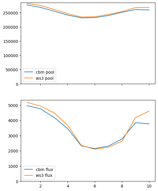
4.11.5. Compare embedded carbon anticipation function to original CBM model
The new ws3 embedded carbon anticipation function is a simplified version of the original CBM model, so we expect it will produce highly correlated but somewhat offset results from the original libcbm model.
We can verify this by comparing carbon output from both models side-by-side.
We start by defining a utility function that runs libcbm, compiles libcbm and ws3 carbon pool and flux data into analogous tables, and plots results.
[46]:
def compare_ws3_cbm(pools=biomass_pools, fluxes=annual_process_fluxes,
                    cbm_x_shift=False,
                    ws3_pool_coeff=1., ws3_flux_coeff=1.,
                    ws3_pool_const=0., ws3_flux_const=0.):
    sit_config, sit_tables = fm.to_cbm_sit(softwood_volume_yname="swdvol",
                                           hardwood_volume_yname="hwdvol",
                                           admin_boundary="British Columbia",
                                           eco_boundary="Montane Cordillera",
                                           disturbance_type_mapping=disturbance_type_mapping)
    n_steps = 100
    cbm_output = run_cbm(sit_config, sit_tables, n_steps, plot=False)
    pi = cbm_output.classifiers.to_pandas().merge(cbm_output.pools.to_pandas(),
                                                  left_on=["identifier", "timestep"],
                                                  right_on=["identifier", "timestep"])
    fi = cbm_output.classifiers.to_pandas().merge(cbm_output.flux.to_pandas(),
                                                  left_on=["identifier", "timestep"],
                                                  right_on=["identifier", "timestep"])
    if cbm_x_shift:
        df_cbm = pd.DataFrame({"period":pi["timestep"] * 0.1,
                           "pool":pi[pools].sum(axis=1),
                           "flux":fi[fluxes].sum(axis=1)}).groupby("period").sum().iloc[1::10, :].reset_index()
        df_cbm["period"] = (df_cbm["period"] - 0.1 + 1.0).astype(int)
    else:
        df_cbm = pd.DataFrame({"period":pi["timestep"] * 0.1,
                           "pool":pi[pools].sum(axis=1),
                           "flux":fi[fluxes].sum(axis=1)}).groupby("period").sum().iloc[10::10, :].reset_index()
        df_cbm["period"] = (df_cbm["period"]).astype(int)

    df_ws3 = pd.DataFrame({"period":fm.periods,
                           "pool":[sum(fm.inventory(period, pool) for pool in pools) for period in fm.periods],
                           "flux":[sum(fm.inventory(period, flux) for flux in fluxes) for period in fm.periods],
                           "ha":[fm.compile_product(period, "1.", acode="harvest") for period in fm.periods]})
    fix, ax = plt.subplots(2, 1, figsize=(6, 8), sharex=True)
    ax[0].plot(df_cbm["period"], df_cbm["pool"], label="cbm pool")
    ax[0].plot(df_ws3["period"], df_ws3["pool"] * ws3_pool_coeff + ws3_pool_const, label="ws3 pool")
    ax[1].plot(df_cbm["period"], df_cbm["flux"], label="cbm flux")
    ax[1].plot(df_ws3["period"], df_ws3["flux"] * ws3_flux_coeff + ws3_flux_const, label="ws3 flux")
    ax[0].legend()
    ax[1].legend()
    ax[0].set_ylim(0, None)
    ax[1].set_ylim(0, None)
    return pi, fi, df_ws3, df_cbm
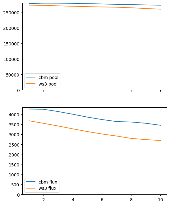
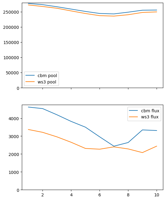
First we run a no-disturbance scenario (i.e., just growth). This should almost perfectly match what we ran through the CBM in the first place to create the carbon yield curves, so we expect there should be a very close match between ws3 and libcbm output for both stocks and fluxes.
[47]:
from util import compile_scenario, plot_scenario
[48]:
fm.reset()
fm.grow()
[49]:
df = compile_scenario(fm)
plot_scenario(df)
[49]:
(<Figure size 1200x400 with 3 Axes>,
 array([<Axes: title={'center': 'Harvested area (ha)'}>,
        <Axes: title={'center': 'Harvested volume (m3)'}>,
        <Axes: title={'center': 'Growing Stock (m3)'}>], dtype=object))
[50]:
pools = biomass_pools + dom_pools + products_pools
fluxes = decay_emissions_fluxes
[51]:
pi, fi, df_ws3, df_cbm = compare_ws3_cbm(pools=pools, fluxes=fluxes)
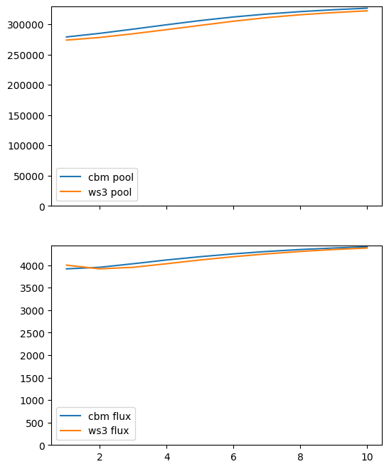
Looks pretty good!
Next, simulate some harvesting.
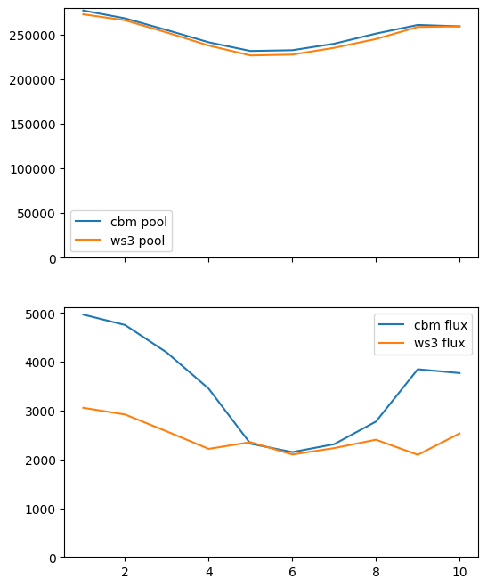
Next, we use the schedule_harvest_areacontrol function defined in the local util module to simulate some harvesting in all periods. We expect there will be more of a gap between ws3 and libcbm carbon estimates, although we still expect ws3 output to be highly correlated with libcbm.
[52]:
fm.reset()
[53]:
from util import schedule_harvest_areacontrol
[54]:
sch = schedule_harvest_areacontrol(fm)
[55]:
df = compile_scenario(fm)
plot_scenario(df)
[55]:
(<Figure size 1200x400 with 3 Axes>,
 array([<Axes: title={'center': 'Harvested area (ha)'}>,
        <Axes: title={'center': 'Harvested volume (m3)'}>,
        <Axes: title={'center': 'Growing Stock (m3)'}>], dtype=object))
[56]:
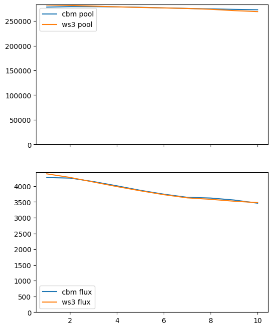
pi, fi, df_ws3, df_cbm = compare_ws3_cbm(pools=pools, fluxes=fluxes)
As expected, when we include harvesting disturbances in our simulation ws3 carbon indicators diverge from corresponding libcbm indicators. The gaps for stocks and fluxes are substantial (and of different magnitudes), but output from both models is hightly correlated. So even with some estimations error, we could likely still use these carbon indicators to define optimization problems in ws3 and get a useful response from the model.
[57]:
df_ws3
[57]:
| period | pool | flux | ha | |
|---|---|---|---|---|
| 0 | 1 | 273038.224079 | 3684.318154 | 103.411088 |
| 1 | 2 | 272183.317438 | 3555.014049 | 105.655079 |
| 2 | 3 | 270757.425489 | 3423.239007 | 103.411088 |
| 3 | 4 | 269290.984414 | 3279.680491 | 103.411088 |
| 4 | 5 | 268189.415203 | 3145.807922 | 103.411088 |
| 5 | 6 | 267189.591266 | 3022.501985 | 103.411088 |
| 6 | 7 | 266209.886837 | 2922.140693 | 103.411088 |
| 7 | 8 | 264538.269595 | 2802.888808 | 114.043292 |
| 8 | 9 | 261988.973856 | 2742.978337 | 114.043292 |
| 9 | 10 | 260038.625703 | 2699.396679 | 114.043292 |
[58]:
pool_corr = (df_cbm["pool"] / df_ws3["pool"]).mean()
pool_corr
[58]:
np.float64(1.0349424535173106)
[59]:
flux_corr = ((df_cbm["flux"] - df_ws3["flux"]) / df_ws3["ha"]).mean()
flux_corr
[59]:
np.float64(6.833749380341729)
Apply correction.
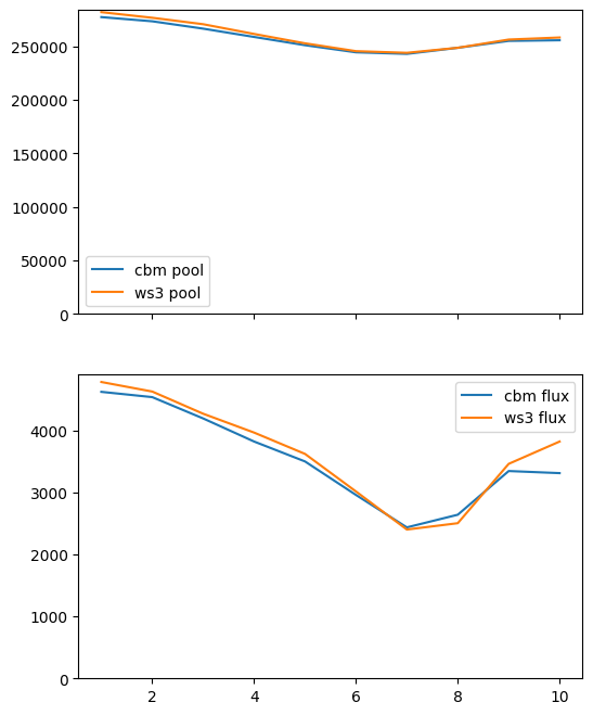
[60]:
pi, fi, df_ws3, df_cbm = compare_ws3_cbm(pools=pools, fluxes=fluxes,
                                         ws3_pool_coeff=pool_corr,
                                         ws3_flux_const=flux_corr*df_ws3["ha"])
Looking good!
Schedule some more harvesting on top of previous solution, to see how stable the gaps are. Not super important what the exact harvest pattern is here, as long as it is distinct from the previous scenario.
[61]:
sch = schedule_harvest_areacontrol(fm)
[62]:
df = compile_scenario(fm)
plot_scenario(df)
[62]:
(<Figure size 1200x400 with 3 Axes>,
 array([<Axes: title={'center': 'Harvested area (ha)'}>,
        <Axes: title={'center': 'Harvested volume (m3)'}>,
        <Axes: title={'center': 'Growing Stock (m3)'}>], dtype=object))
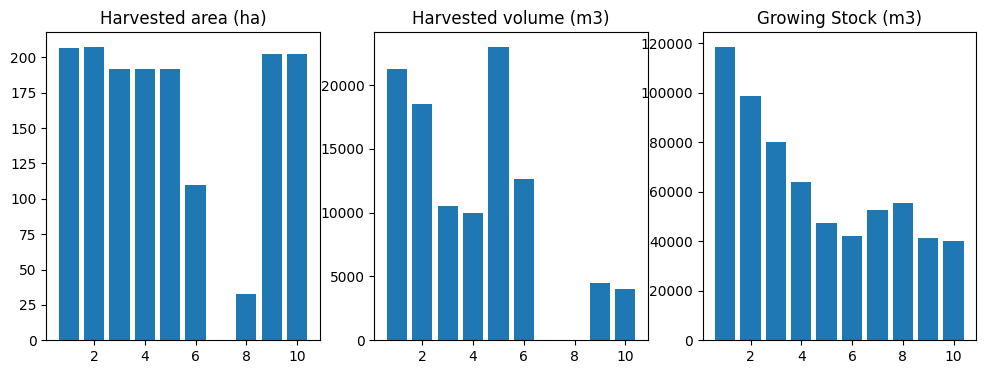
No correction.
[63]:
pi, fi, df_ws3, df_cbm = compare_ws3_cbm(pools=pools, fluxes=fluxes)
With correction.
[64]:
pi, fi, df_ws3, df_cbm = compare_ws3_cbm(pools=pools, fluxes=fluxes,
                                         ws3_pool_coeff=pool_corr,
                                         ws3_flux_const=flux_corr*df_ws3["ha"])
Very nice! Now try again with more harvesting, to test stability of the correction hack.
[65]:
sch = schedule_harvest_areacontrol(fm)
[66]:
df = compile_scenario(fm)
plot_scenario(df)
[66]:
(<Figure size 1200x400 with 3 Axes>,
 array([<Axes: title={'center': 'Harvested area (ha)'}>,
        <Axes: title={'center': 'Harvested volume (m3)'}>,
        <Axes: title={'center': 'Growing Stock (m3)'}>], dtype=object))
No correction.
[67]:
pi, fi, df_ws3, df_cbm = compare_ws3_cbm(pools=pools, fluxes=fluxes)
With correction.
[68]:
pi, fi, df_ws3, df_cbm = compare_ws3_cbm(pools=pools, fluxes=fluxes,
                                         ws3_pool_coeff=pool_corr,
                                         ws3_flux_const=flux_corr*df_ws3["ha"])
Note that this correction hack is not guaranteed to work for all datasets, but might constitute a good start if you want to apply develop a single correction hack that could be applied to all carbon and flux indicators in your ws3 model (across all scenarios). The way we implemented this would work reasonably well as a post hoc correction on ws3 model output (e.g., for reporting), but does not correct the carbon indicators inside the model (so they would still be a bit wonky and
might distort harvesting solutions, e.g., if we included one or more wonky carbon indicators in an optimization problem).
You could easily implement a similar pool correction inside ws3 by scaling all carbon pool yield curves by an appropriate coefficient.
The correction we applied to the flux estimates would be less intuitive to implement. To implement this correction inside an optimizaiton problem, you would likely have to define the appropriate coeff_func function to return something like \(x + (Cxy)\), where \(x\) is something like fm.inventory(..., yname='flux_yname', ...), \(y\) is something like (fm.compile_product(..., expr='1.', acode='harvest', ...) and \(C\) is the flux correction coefficient (calculated
similary to how we did it above, but then divided by the total system flux in ws3). Might get a bit messy, and may not be necessary at all depending on what you are trying to do (and why).
The post hoc calibration should work well enough for reporting purposes (or to confirm that “optimizing” for carbon in a ws3 scenario actually did more good than harm, which is not a given).